Lecture 10
More on Gaussian Processes and Kernels
Noisy regression
Last time, we had observed that the values of the function were uncorrupted by noise.
Rather than observe the true function values, {\color{orange}{f_n}}, we observe {\color{yellow}{t_n}}, where {\color{yellow}{t_n}} = {\color{orange}{f_n}} + \epsilon_{n}, \; \; \; \textsf{where} \; \; \; p \left( \epsilon_{n} \right) = \mathcal{N}\left(0, \sigma^2 \right)
Setting {\color{yellow}{\mathbf{t}}} = \left[ {\color{yellow}{t_1, t_2, \ldots, t_{N}}} \right]^{T} as before, we have p \left( {\color{yellow}{\mathbf{t}}} | {\color{orange}{\mathbf{f}}}, \sigma^2 \right) = \mathcal{N} \left({\color{orange}{\mathbf{f}}}, \sigma^2 \mathbf{I}_{N} \right).
Integrating {\color{orange}{\mathbf{f}}} out and placing a prior directly on {\color{yellow}{\mathbf{t}}} leads to p \left( {\color{yellow}{\mathbf{t}}} | \sigma^2 \right) = \int p \left( {\color{yellow}{\mathbf{t}}} | {\color{orange}{\mathbf{f}}}, \sigma^2 \right) p \left( {\color{orange}{\mathbf{f}}} \right) d {\color{orange}{\mathbf{f}}} = \mathcal{N} \left(\mathbf{0}, \mathbf{C} + \sigma^2 \mathbf{I}_{N} \right)
Noisy regression
Normally, we are interested in predicting {\color{orange}{\mathbf{f}}}^{\ast}, the underlying function rather than {\color{yellow}{\mathbf{t}}}^{\ast}, the corrupted signal value.
The joint density (as before) is given by p \left( {\color{orange}{\mathbf{\hat{f}}}} | \sigma^2 \right) = \mathcal{N} \left( \mathbf{0}, \left[\begin{array}{cc} \mathbf{C} + \sigma^2 \mathbf{I}_{N} & \mathbf{R} \\ \mathbf{R}^{T} & \mathbf{C}^{\ast} \end{array}\right] \right) where \mathbf{\hat{{\color{orange}{\mathbf{f}}}}} = \left[ {\color{yellow}{\mathbf{t}}}, {\color{orange}{\mathbf{f}}}^{\ast} \right]^{T}.
Note that if we wished to predict {\color{yellow}{\mathbf{t}}}^{\ast}, the bottom right matrix block would be \mathbf{C}^{\ast} + \sigma^2 \mathbf{I}_{L} instead of \mathbf{C}^{\ast}.
Noisy regression
- We obtain the predictive conditional distribution p \left( {\color{orange}{\mathbf{f}}}^{\ast} | {\color{yellow}{\mathbf{t}}}, \sigma^2 \right), where \begin{aligned} p \left( {\color{orange}{\mathbf{f}}}^{\ast} | {\color{yellow}{\mathbf{t}}}, \sigma^2 \right) & = \mathcal{N} \left( \boldsymbol{\mu}^{\ast}, \boldsymbol{\Sigma}^{\ast} \right) \\ \boldsymbol{\mu}^{\ast} = \mathbf{R}^{T} \left( \mathbf{C} + \sigma^2 \mathbf{I}_{N} \right)^{-1} {\color{yellow}{\mathbf{t}}}, \; \; & \; \; \boldsymbol{\Sigma}^{\ast} = \mathbf{C}^{\ast} - \mathbf{R}^{T} \left( \mathbf{C} + \sigma^2 \mathbf{I}_{N} \right)^{-1}\mathbf{R} \end{aligned}
Noisy regression
- We can reach this predicitive distribution through an alternative route. This derivation will be useful when we study non-Gaussian likelihoods (e.g., required for classification problems). Can write p \left( {\color{orange}{\mathbf{f}}}^{\ast} | {\color{yellow}{\mathbf{t}}}, \sigma^2 \right) = \int \underbrace{p \left( {\color{orange}{\mathbf{f}}}^{\ast} | {\color{orange}{\mathbf{f}}} \right)}_{\textsf{Noise-free GP (see lecture 9)}} p \left( {\color{orange}{\mathbf{f}}} | {\color{yellow}{\mathbf{t}}}, \sigma^2 \right) d {\color{orange}{\mathbf{f}}}
- The first term (from last time) is: p \left( {\color{orange}{\mathbf{f}}}^{\ast} | {\color{orange}{\mathbf{f}}} \right) = \mathcal{N} \left(\mathbf{R}^{T} \mathbf{C}^{-1} {\color{orange}{\mathbf{f}}}, \mathbf{C}^{\ast} - \mathbf{R}^{T} \mathbf{C}^{-1} \mathbf{R} \right)
Noisy regression
- Second term can be computed via Bayes’ rule: \begin{aligned} p \left( {\color{orange}{\mathbf{f}}} | {\color{yellow}{\mathbf{t}}}, \sigma^2 \right) & \propto \mathcal{N}\left( {\color{yellow}{\mathbf{t}}} | {\color{orange}{\mathbf{f}}} , \sigma^2 \mathbf{I} \right) \mathcal{N} \left( {\color{orange}{\mathbf{f}}} | \mathbf{0} , \mathbf{C} \right) \\ & \propto exp \left\{ -\frac{1}{2} \left( {\color{yellow}{\mathbf{t}}} - {\color{orange}{\mathbf{f}}} \right)^{T} \left( \sigma^2 \mathbf{I}\right)^{-1} \left( {\color{yellow}{\mathbf{t}}} - {\color{orange}{\mathbf{f}}} \right) \right\} \; exp \left\{ -\frac{1}{2} {\color{orange}{\mathbf{f}}}^{T} \mathbf{C}^{-1} {\color{orange}{\mathbf{f}}} \right\} \\ & = \mathcal{N} \left( \underbrace{\frac{1}{\sigma^2} \boldsymbol{\Sigma}_{{\color{orange}{\mathbf{f}}}} {\color{yellow}{\mathbf{t}}}}_{\boldsymbol{\mu}_{{\color{orange}{\mathbf{f}}}} }, \underbrace{\left[ \mathbf{C}^{-1} + \frac{1}{\sigma^2} \mathbf{I} \right]^{-1}}_{\boldsymbol{\Sigma}_{{\color{orange}{\mathbf{f}}}}} \right) \end{aligned}
Noisy regression
- This leads to \begin{aligned} p \left( {\color{orange}{\mathbf{f}}}^{\ast} | {\color{yellow}{\mathbf{t}}} , \sigma^2 \right) & = \mathcal{N}\left( \mathbf{R}^{T} \mathbf{C}^{-1} \boldsymbol{\mu}_{{\color{orange}{\mathbf{f}}}} , \mathbf{C}^{\ast} - \mathbf{R}^{T} \mathbf{C}^{-1} \mathbf{R} + \mathbf{R}^{T} \mathbf{C}^{-1} \boldsymbol{\Sigma}_{{\color{orange}{\mathbf{f}}}} \mathbf{C}^{-1} \mathbf{R} \right)\\ & = \mathcal{N} \left(\mathbf{R}^{T} \mathbf{C}^{-1} {\color{orange}{\mathbf{f}}}, \mathbf{C}^{\ast} - \mathbf{R}^{T} \left( \mathbf{C} + \sigma^{2} \mathbf{I}_{N} \right)^{-1} \mathbf{R} \right) \end{aligned}
Kernels
Last time we briefly introduced a covariance function or a kernel. Formally, we define it as {\color{lime}{k}} : \mathcal{X} \times \mathcal{X} \rightarrow \mathbb{R} which maps a pair of inputs \mathbf{x}, \mathbf{x}' \in \mathcal{X} from some input space to the real line \mathbb{R}.
Schaback and Wendland state that \mathcal{X} should be general enough to allow ``Shakespeare texts or X-ray images’’.
Kernels occuring in machine learning and general, but they can take a special form tailored for the applications.
Kernels
Not all functions of the form {\color{lime}{k}} \left( \mathbf{x}, \mathbf{x}' \right) are valid covariance functions.
Covariance functions must yield symmetric positive (semi-) definite matrices, i.e., if \mathbf{C}_{ij} = {\color{lime}{k}} \left( \mathbf{x}, \mathbf{x}' \right), then \mathbf{C} = \mathbf{C}^{T} \; \;\textsf{and} \; \; \mathbf{x}^{T} \mathbf{C} \mathbf{x} \geq 0 \; (\textsf{for all} \; \mathbf{x} \neq 0 ).
A covariance function is stationary if {\color{lime}{k}} \left( \mathbf{x}, \mathbf{x}' \right) depends only on the difference in inputs, i.e., {\color{lime}{k}} \left( \mathbf{x}, \mathbf{x}' \right) = {\color{lime}{k}} \left( \mathbf{x} - \mathbf{x}' \right), and is said to be isotropic (rotationally invariant) if it depends on the norm of the differences, i.e., {\color{lime}{k}} \left( \mathbf{x}, \mathbf{x}' \right) = {\color{lime}{k}} \left( || \mathbf{x} - \mathbf{x}'|| \right).
Kernels
Please see RW for a list of valid kernel functions. Additionally, note that one can create bespoke kernels.
In general, following the rules of symmetric PSD matrices, we have:
- Products of two kernels: {\color{lime}{k}} \left( \mathbf{x}, \mathbf{x}' \right) = {\color{lime}{k}_{A}} \left( \mathbf{x}, \mathbf{x}' \right) \times {\color{lime}{k}_{B}} \left( \mathbf{x}, \mathbf{x}' \right)
- Scaling a kernel: {\color{lime}{k}} \left( \mathbf{x}, \mathbf{x}' \right) = g\left(\mathbf{x} \right){\color{lime}{k}_{A}} \left( \mathbf{x}, \mathbf{x}' \right) g\left(\mathbf{x}' \right), for an arbitrary g.
- Sum of two kernels: {\color{lime}{k}} \left( \mathbf{x}, \mathbf{x}' \right) = {\color{lime}{k}_{A}} \left( \mathbf{x}, \mathbf{x}' \right) + {\color{lime}{k}_{B}} \left( \mathbf{x}, \mathbf{x}' \right)
- Other operations, as captured in Bishop; see next slide.
Kernels
 Bishop, C., (2006) Pattern Recognition and Machine Learning, Springer.
Kernels
In your reading of Chapter 2 of RW, you have / will come across the kernel trick.
 Rasmussen, C., Williams, C., (2006) Gaussian Processes for Machine Learning, MIT.
Kernels
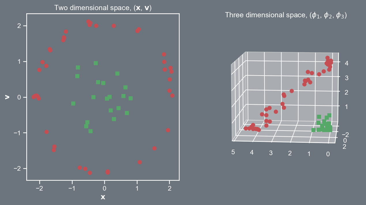
Consider a quadratic kernel in \mathbb{R}^{2}, where \mathbf{x} = \left(x_1, x_2 \right)^{T} and \mathbf{v} = \left(v_1, v_2 \right)^{T}. \begin{aligned} {\color{lime}{k}} \left( \mathbf{x}, \mathbf{v} \right) = \left( \mathbf{x}^{T} \mathbf{v} \right)^2 & = \left( \left[\begin{array}{cc} x_{1} & x_{2}\end{array}\right]\left[\begin{array}{c} v_{1}\\ v_{2} \end{array}\right] \right)^2 \\ & = \left( x_1^2 v_1^2 + 2 x_1 x_2 v_1 v_2 + x_2^2 v_2^2\right) \\ & = \left[\begin{array}{ccc} x^2_{1} & \sqrt{2} x_1 x_2 & x_2^2 \end{array}\right]\left[\begin{array}{c} v_{1}^2\\ \sqrt{2}v_1 v_2 \\ v_{2}^2 \end{array}\right] \\ & = \phi \left( \mathbf{x} \right)^{T} \phi \left( \mathbf{v} \right). \end{aligned} where \phi \left( \cdot \right) \in \mathbb{R}^{3}.
Kernels
This kernel trick permits us to transform the data to higher dimensions.
Now if we try to linearly separate the data it is far easier, i.e., our decision boundaries will be hyperplanes in \mathbb{R}^{3}.
Kernels
- Qualitatively, a kernel dictates the function space. Some properties of interest might be:
- Is the kernel infinitely differentiable?
- Is the kernel periodic?
- Is the kernel symmetric about a certain axis?
- Is the kernel non-stationary?
- While there are many characterizations of kernels, we will focus on (i) structured kernels; (ii) spectral kernels; (iii) deep kernels over the next few lectures.
L10 | More on Gaussian Processes and Kernels