Lecture 6

Linear modelling

The three model levels

In this lecture, we will explore three distinct but related flavors of modelling.

Linear least squares model
Gaussian noise model (introducing the idea of likelihood)
Full Bayesian treatment (next time!)

Much of the exposition shown here is based on the first three chapters of Rogers and Girolami’s, A First Course in Machine Learning.

Linear least squares

Consider the data shown in the plot below. It shows the winning times for the men’s 100 meter race at the Summer Olympics for many years.

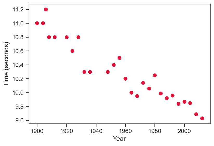
Our goal will be to fit a model to this data. To begin, we will consider a linear model, i.e., t = f \left( x; {\color{blue}{w_0}}, {\color{blue}{w_1}} \right) = {\color{blue}{w_0}} + {\color{blue}{w_1}} x where x is the year and t is the winning time.
{\color{blue}{w_0}} and {\color{blue}{w_1}} are unknown model parameters that we need to ascertain.
Good sense would suggest that the best line passes as closely as possible through all the data points on the left.

Linear least squares

Defining a good model

One common strategy for defining this is based on the squared distance between the truth and the model. Thus, for a given year, t_i, this is written as: \mathcal{L}_{i} = \left( t_i - f \left( x_i; {\color{blue}{w_0}}, {\color{blue}{w_1}} \right) \right)^2.
However, as we want a model that fits well across all the data, we may consider the average across the entire data set, i.e., all N data points. This is given by: \mathcal{L} = \frac{1}{N} \sum_{i=1}^{N} \mathcal{L}_{i} = \frac{1}{N} \sum_{i=1}^{N} \left( t_i - f \left( x_i; {\color{blue}{w_0}}, {\color{blue}{w_1}} \right) \right)^2
Note that this loss function is always positive, and the lower it is the better! Finding optimal values for {\color{blue}{w_0}}, {\color{blue}{w_1}} can be expressed as \underset{{\color{blue}{w_0}}, {\color{blue}{w_1}}}{argmin} \; \; \frac{1}{N} \sum_{i=1}^{N} \left( t_i - f \left( x_i; {\color{blue}{w_0}}, {\color{blue}{w_1}} \right) \right)^2

Linear least squares

Matrix-vector notation

It will be very useful to work with vectors and matrices. For convenience, we define: \mathbf{X}=\left[\begin{array}{cc} 1 & x_{1}\\ 1 & x_{2}\\ \vdots & \vdots\\ 1 & x_{N} \end{array}\right] = \left[\begin{array}{c} \mathbf{x}_{1}^{T}\\ \mathbf{x}_{2}^{T}\\ \vdots \\ \mathbf{x}_{N}^{T} \end{array}\right], \; \; \; \; \; \mathbf{t} =\left[\begin{array}{c} t_{1}\\ t_{2}\\ \vdots\\ t_{N} \end{array}\right], \; \; \; \; \; \mathbf{{\color{blue}{w}}} = \left[\begin{array}{c} {\color{blue}{w_0}}\\ {\color{blue}{w_1}} \end{array}\right]
The loss function from the prior slide is equivalent to writing \mathcal{L} = \frac{1}{N} \left( \mathbf{t} - \mathbf{X} \mathbf{{\color{blue}{w}}} \right)^{T} \left( \mathbf{t} - \mathbf{X} \mathbf{{\color{blue}{w}}} \right).
This can be expanded to yield \mathcal{L} = \frac{1}{N} \left( \mathbf{t}^{T} - \left( \mathbf{X} \mathbf{{\color{blue}{w}}} \right)^T \right)\left( \mathbf{t} - \mathbf{X} \mathbf{{\color{blue}{w}}} \right) = \frac{1}{N} \left[ \mathbf{t}^{T} \mathbf{t} - 2 \mathbf{t}^{T} \mathbf{X} \mathbf{{\color{blue}{w}}} + \mathbf{{\color{blue}{w}}}^T \mathbf{X}^{T} \mathbf{X} \mathbf{{\color{blue}{w}}} \right]

Linear least squares

Minimizing the loss

As our objective is to minimize the loss, the obvious idea is to find out for which \mathbf{{\color{blue}{w}}}, the derivative of the loss function, \partial \mathcal{L} / \partial \mathbf{{\color{blue}{w}}}, goes to zero.
Note that in practice, we refer to these points as turning points as they may equally correspond to maxima, minima, or saddle points. A positive second derivative is a sure sign of a minima.
Prior to working out the derivatives, it will be useful to take note of the following identities on the left below.

g \left( \mathbf{{\color{red}{v}}} \right)	\partial g / \partial \mathbf{{\color{red}{v}}}
\mathbf{{\color{red}{v}}}^{T}\mathbf{x}	\mathbf{x}
\mathbf{x}^{T} \mathbf{{\color{red}{v}}}	\mathbf{x}
\mathbf{{\color{red}{v}}}^{T} \mathbf{{\color{red}{v}}}	2\mathbf{{\color{red}{v}}}
\mathbf{{\color{red}{v}}}^{T} \mathbf{C} \mathbf{{\color{red}{v}}}	2\mathbf{C} \mathbf{{\color{red}{v}}}

The derivative of the loss function is given by \frac{\partial \mathcal{L}}{\partial \mathbf{{\color{blue}{w}}}} = - \frac{2}{N} \mathbf{X}^{T} \mathbf{t} + \frac{2}{N} \mathbf{X}^{T} \mathbf{X} \mathbf{{\color{blue}{w}}}
Setting the derivative to zero, we have \mathbf{X}^{T} \mathbf{X} \mathbf{{\color{blue}{w}}} = \mathbf{X}^{T} \mathbf{t} \; \; \; \Rightarrow \; \; \; \hat{\mathbf{{\color{blue}{w}}}} = \left( \mathbf{X}^{T} \mathbf{X} \right)^{-1} \mathbf{X}^{T} \mathbf{t} where \hat{\mathbf{{\color{blue}{w}}}} represents the value of \mathbf{{\color{blue}{w}}} that minimizes the loss.

import pandas as pd
import numpy as np
import matplotlib.pyplot as plt
import seaborn as sns
sns.set(font_scale=1.0)
sns.set_style("white")
sns.set_style("ticks")
palette = sns.color_palette('deep')

df = pd.read_csv('notebooks/data/data100m.csv')
df.columns=['Year', 'Time']
N = df.shape[0]

max_year, min_year = df['Year'].values.max() , df['Year'].values.min()

x = (df['Year'].values.reshape(N,1) - min_year)/(max_year - min_year)
t = df['Time'].values.reshape(N,1)
X_func = lambda u : np.hstack([np.ones((u.shape[0],1)), u])
X = X_func(x)
w_hat = np.linalg.inv(X.T @ X) @ X.T @ t
loss_func = 1./N * (t - X @ w_hat).T @ (t - X @ w_hat)

xgrid = np.linspace(0, 1, 100).reshape(100,1)
Xg = X_func(xgrid)
time_grid = Xg @ w_hat

fig = plt.figure(figsize=(6,4))
plt.plot(df['Year'].values, df['Time'].values, 'o', color='crimson', label='Data')
plt.plot(xgrid*(max_year - min_year) + min_year, time_grid, '-', color='dodgerblue', label='Model')
plt.xlabel('Year')
plt.ylabel('Time (seconds)')
loss_title = r'Loss function, $\mathcal{L}=$'+str(np.around(float(loss_func), 5))+'; \t norm of $\hat{\mathbf{w}}$='+str(np.around(float(np.linalg.norm(w_hat,2)), 3))
plt.title(loss_title)
plt.legend()
plt.savefig('olympics_0.png', dpi=150, bbox_inches='tight')
plt.close()

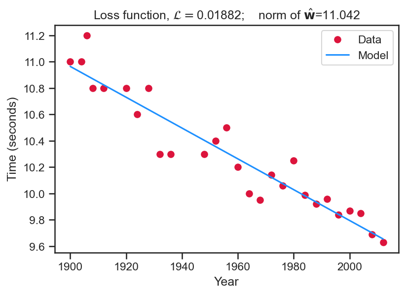
For this result we set \mathbf{X}=\left[\begin{array}{cc} 1 & x_{1}\\ 1 & x_{2}\\ \vdots & \vdots\\ 1 & x_{N} \end{array}\right] and solve for \hat{\mathbf{{\color{blue}{w}}}} = \left( \mathbf{X}^{T} \mathbf{X} \right)^{-1} \mathbf{X}^{T} \mathbf{t}.

Once these weights are obtained, we can extrapolate (blue line) over the years.

Note the graph title shows the loss function value and the L_2 norm, \left\Vert\hat{\mathbf{{\color{blue}{w}}}}\right\Vert_{2}.

Linear least squares

Plot
Code

import pandas as pd
import numpy as np
import matplotlib.pyplot as plt
import seaborn as sns
sns.set(font_scale=1.0)
sns.set_style("white")
sns.set_style("ticks")
palette = sns.color_palette('deep')

df = pd.read_csv('notebooks/data/data100m.csv')
df.columns=['Year', 'Time']
N = df.shape[0]

max_year, min_year = df['Year'].values.max() , df['Year'].values.min()

x = (df['Year'].values.reshape(N,1) - min_year)/(max_year - min_year)
t = df['Time'].values.reshape(N,1)
X_func = lambda u : np.hstack([np.ones((u.shape[0],1)), u , u**2, u**3])
X = X_func(x)
w_hat = np.linalg.inv(X.T @ X) @ X.T @ t
loss_func = 1./N * (t - X @ w_hat).T @ (t - X @ w_hat)

xgrid = np.linspace(0, 1, 100).reshape(100,1)
Xg = X_func(xgrid)
time_grid = Xg @ w_hat

fig = plt.figure(figsize=(6,4))
plt.plot(df['Year'].values, df['Time'].values, 'o', color='crimson', label='Data')
plt.plot(xgrid*(max_year - min_year) + min_year, time_grid, '-', color='dodgerblue', label='Model')
plt.xlabel('Year')
plt.ylabel('Time (seconds)')
loss_title = r'Loss function, $\mathcal{L}=$'+str(np.around(float(loss_func), 5))+'; \t norm of $\hat{\mathbf{w}}$='+str(np.around(float(np.linalg.norm(w_hat,2)), 3))
plt.title(loss_title)
plt.legend()
plt.savefig('olympics_3.png', dpi=150, bbox_inches='tight')
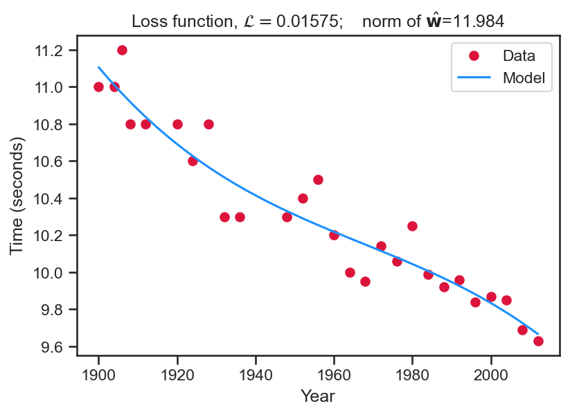
plt.close()

For this result we set \mathbf{X}=\left[\begin{array}{cccc} 1 & x_{1} & x_{1}^2 & x_{1}^3\\ 1 & x_{2} & x_{2}^2 & x_{2}^3\\ \vdots & \vdots & \vdots & \vdots\\ 1 & x_{N} & x_{N}^2 & x_{N}^3 \end{array}\right] and solve for \hat{\mathbf{{\color{blue}{w}}}} = \left( \mathbf{X}^{T} \mathbf{X} \right)^{-1} \mathbf{X}^{T} \mathbf{t}.

Once these weights are obtained, we can extrapolate (blue line) over the years.

Note the graph title shows the loss function value and the L_2 norm, \left\Vert\hat{\mathbf{{\color{blue}{w}}}}\right\Vert_{2}.

Linear least squares

Plot
Code

import pandas as pd
import numpy as np
import matplotlib.pyplot as plt
import seaborn as sns
sns.set(font_scale=1.0)
sns.set_style("white")
sns.set_style("ticks")
palette = sns.color_palette('deep')

df = pd.read_csv('notebooks/data/data100m.csv')
df.columns=['Year', 'Time']
N = df.shape[0]

max_year, min_year = df['Year'].values.max() , df['Year'].values.min()

x = (df['Year'].values.reshape(N,1) - min_year)/(max_year - min_year)
t = df['Time'].values.reshape(N,1)
X_func = lambda u : np.hstack([np.ones((u.shape[0],1)), u , u**2, u**3])
X = X_func(x)
w_hat = np.linalg.inv(X.T @ X) @ X.T @ t
loss_func = 1./N * (t - X @ w_hat).T @ (t - X @ w_hat)

xgrid = np.linspace(0, 1, 100).reshape(100,1)
Xg = X_func(xgrid)
time_grid = Xg @ w_hat

fig = plt.figure(figsize=(6,4))
plt.plot(df['Year'].values, df['Time'].values, 'o', color='crimson', label='Data')
plt.plot(xgrid*(max_year - min_year) + min_year, time_grid, '-', color='dodgerblue', label='Model')
plt.xlabel('Year')
plt.ylabel('Time (seconds)')
loss_title = r'Loss function, $\mathcal{L}=$'+str(np.around(float(loss_func), 5))+'; \t norm of $\hat{\mathbf{w}}$='+str(np.around(float(np.linalg.norm(w_hat,2)), 3))
plt.title(loss_title)
plt.legend()
plt.savefig('olympics_8.png', dpi=150, bbox_inches='tight')
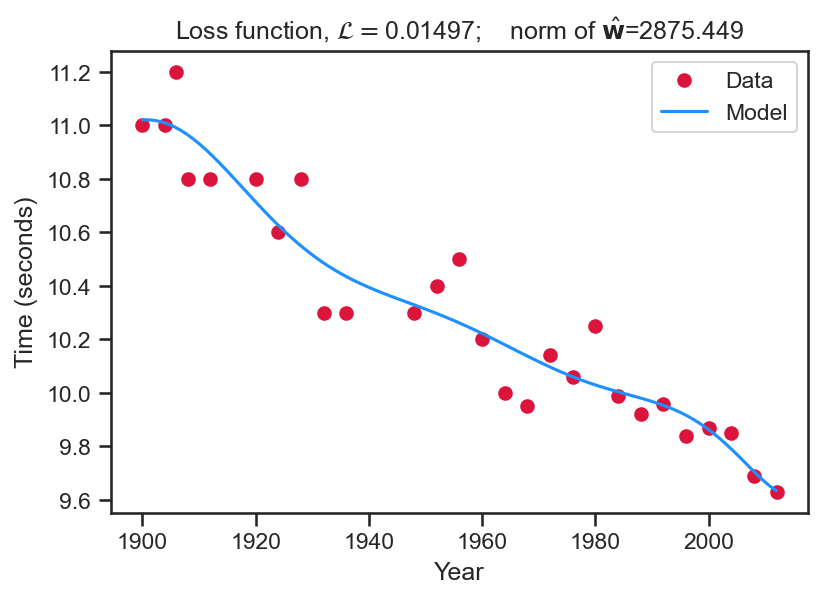
plt.close()

For this result we set \mathbf{X}=\left[\begin{array}{cccccc} 1 & x_{1} & x_{1}^2 & x_{1}^3 & \ldots & x_{1}^{8} \\ 1 & x_{2} & x_{2}^2 & x_{2}^3 & \ldots & x_{2}^{8} \\ \vdots & \vdots & \vdots & \vdots & \ldots & \vdots \\ 1 & x_{N} & x_{N}^2 & x_{N}^3 & \ldots & x_{N}^{8} \\ \end{array}\right] and solve for \hat{\mathbf{{\color{blue}{w}}}} = \left( \mathbf{X}^{T} \mathbf{X} \right)^{-1} \mathbf{X}^{T} \mathbf{t}.

Once these weights are obtained, we can extrapolate (blue line) over the years.

Note the graph title shows the loss function value and the L_2 norm, \left\Vert\hat{\mathbf{{\color{blue}{w}}}}\right\Vert_{2}.

Linear least squares

With regularization

There is clearly a trade-off between the:
- Complexity of the model in terms of the number of weights, and
- the value of the loss function.
There is also the risk of over-fitting to the data. For instance, if we had only 9 data points, then the last model would have interpolated each point, at the risk of not being generalizable.
As we do not want our model to be too complex, there are two relatively simple recipes:
- Split the data into test and train (your homework!)
- Add a regularization term, i.e., \mathcal{L} = \mathcal{L} + \lambda \mathbf{{\color{blue}{w}}}^{T} \mathbf{{\color{blue}{w}}} where \lambda is a constant.

Maximum likelihood

The linear model from before is unable to capture each data point, and there are errors between the true data and the model.
Now we will consider a paradigm where these errors are explicitly modelled.
We consider a model of the form t_j = f \left( \mathbf{x}_{n}; \mathbf{{\color{blue}{w}}} \right) + \epsilon_{n} \; \; \; \epsilon_{n} \sim \mathcal{N}\left(0, \sigma^2 \right), \; \; \; \; \text{where} \; j \in \left[1, N \right] \tag{1}
Recall, we had previously learnt that adding a constant to a Gaussian random variable alters its mean. Thus, the random variable t_j has a probability density function p \left( t_j | \mathbf{x}_{j}, \mathbf{{\color{blue}{w}}}, \sigma^2 \right) = \mathcal{N} \left( \mathbf{{\color{blue}{w}}}^{T} \mathbf{x}_{j} , \sigma^2\right)
Carefully note the conditioning: the probability density function for t_j depends on particular values of \mathbf{x}_{j} and \mathbf{{\color{blue}{w}}}.

Maximum likelihood

Defining the likelihood

If we evaluate the linear model from before, and assume that in Equation 1 \sigma^2 = 0.05, we would find that p \left( t_j | \mathbf{x}_{j} = \left[ 1, 1980 \right]^{T} ,\mathbf{{\color{blue}{w}}} = \left[10.964, -1.31 \right]^{T}, \sigma^2 = 0.05 \right) = \mathcal{N} \left( 10.03, 0.05 \right) This quantity is known as the likelihood of the n-th data point.

Plot
Code

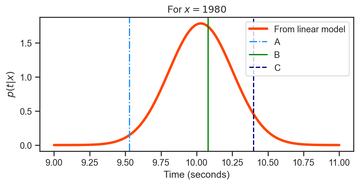
Note that for a continuous random variable t, p\left( t \right) cannot be interpreted as a probability.
The height of the curve to the left tells us how likely it is that we observe a particular t for x=1980.
The most likely is B, followed by C and then A. Note the actual winning time is t_{n}=10.25.
While we obviously cannot change the actual winning time, we can change \mathbf{{\color{blue}{w}}} and \sigma^2 to move the density to make it as high as possible at t=10.25.

import numpy as np
import matplotlib.pyplot as plt
import pandas as pd
from scipy.stats import multivariate_normal

# Get the data 
df = pd.read_csv('notebooks/data/data100m.csv')
df.columns=['Year', 'Time']
N = df.shape[0]
max_year, min_year = df['Year'].values.max() , df['Year'].values.min()
x = (df['Year'].values.reshape(N,1) - min_year)/(max_year - min_year)
t = df['Time'].values.reshape(N,1)
X_func = lambda u : np.hstack([np.ones((u.shape[0],1)), u])
X = X_func(x)
w_hat = np.linalg.inv(X.T @ X) @ X.T @ t

# Specific year!
year_j = 1980
X_j = X_func(np.array( [ (year_j - min_year) / (max_year - min_year) ] ).reshape(1,1) )
time_j = float(X_j @ w_hat)

T_1980 = multivariate_normal(time_j, 0.05)
ti = np.linspace(9, 11, 100)
pt_x = T_1980.pdf(ti)

fig = plt.figure(figsize=(7,3))
plt.plot(ti, pt_x, '-', color='orangered', lw=3, label='From linear model')
plt.axvline(9.53, linestyle='-.', color='dodgerblue', label='A')
plt.axvline(10.08, linestyle='-', color='green', label='B')
plt.axvline(10.40, linestyle='--', color='navy', label='C')
plt.xlabel('Time (seconds)')
plt.ylabel(r'$p \left( t | x \right)$')
plt.title(r'For $x=1980$')
plt.legend()
plt.close()

Maximum likelihood

Defining the likelihood

This idea of finding parameters that can maximize the likelihood is very important in machine learning.
However, in general, we are seldom interested in the likelihood of an isolated data point – we are interested in the likelihood across all the data.
This leads to the conditional distribution across all N data points p \left( t_1, \ldots, t_N | \mathbf{x}_1, \ldots, \mathbf{x}_{N}, \mathbf{{\color{blue}{w}}}, \sigma^2 \right)
If we assume the noise at each data point is independent, this conditional density can be factorized into N separate terms \mathcal{L} = p \left( \mathbf{t} | \mathbf{X}, \mathbf{{\color{blue}{w}}}, \sigma^2 \right) = \prod_{j=1}^{N} p \left( t_j | \mathbf{x}_{j}, \mathbf{{\color{blue}{w}}}, \sigma^2 \right) = \prod_{j=1}^{N} \mathcal{N} \left(\mathbf{{\color{blue}{w}}}^{T} \mathbf{x}_{n} \right). \tag{2}
Note that the t_j values are not completely independent—times have clearly decreased over the years! They are conditionally independent. For a given value of \mathbf{{\color{blue}{w}}} the t_j are independent; otherwise they are not.
We will now maximize the likelihood (see Equation 2 ).

Maximum likelihood

Maximizing the logarithm of the likelihood

Plugging in the definition of a Gaussian probability density function into Equation 2 we arrive at \mathcal{L} = \prod_{j=1}^{N} \frac{1}{\sqrt{2 \pi \sigma^2}} exp \left( -\frac{1}{2 \sigma^2} \left(t_j - f \left( \mathbf{x}_{j}; \mathbf{{\color{blue}{w}}} \right) \right)^2 \right)
Taking the logarithm on both sides and simplifying: log \left( \mathcal{L} \right) = \sum_{j=1}^{N} log \left( \frac{1}{\sqrt{2 \pi \sigma^2}} exp \left( -\frac{1}{2 \sigma^2} \left(t_j - f \left( \mathbf{x}_{j}; \mathbf{{\color{blue}{w}}} \right) \right)^2 \right) \right) = \sum_{j=1}^{N} \left( -\frac{1}{2} log \left( 2 \pi \right) - log \left(\sigma \right) - \frac{1}{2\sigma^2} \left( t_j - f \left(\mathbf{x}_{j}; \mathbf{{\color{blue}{w}}} \right) \right)^2 \right) = -\frac{N}{2} log \left( 2 \pi \right) - N \; log \left( \sigma \right) - \frac{1}{2 \sigma^2} \sum_{j=1}^{N} \left(t_j - f \left(\mathbf{x}_{j}; \mathbf{{\color{blue}{w}}} \right) \right)^2

Maximum likelihood

Maximizing the logarithm of the likelihood

Just as we did earlier, with the least squares solution, we can set the derivative of the logarithm of the loss function to be zero. \frac{\partial \; log \left( \mathcal{L} \right) }{\partial \mathbf{{\color{blue}{w}}}} = \frac{1}{\sigma^2} \sum_{j=1}^{N} \mathbf{x}_{j} \left( t_{j} - \mathbf{x}_{j}^{T} \mathbf{{\color{blue}{w}}} \right) = \frac{1}{\sigma^2} \sum_{j=1}^{N} \mathbf{x}_{j} t_j - \mathbf{x}_{j} \mathbf{x}_{j}^{T} \mathbf{{\color{blue}{w}}} \equiv 0
Just as we did before, we can use matrix vector notation to write this out as

\frac{\partial \; log \left( \mathcal{L} \right) }{\partial \mathbf{{\color{blue}{w}}} } = \frac{1}{\sigma^2} \left( \mathbf{X}^{T} \mathbf{t} - \mathbf{X}^{T} \mathbf{X} \mathbf{{\color{blue}{w}}}\right) = 0

Solving this expression leads to
\mathbf{X}^{T} \mathbf{t} - \mathbf{X}^{T} \mathbf{X} \mathbf{{\color{blue}{w}}} = 0 \Rightarrow \hat{\mathbf{{\color{blue}{w}}}} = \left( \mathbf{X}^{T} \mathbf{X} \right)^{-1} \mathbf{X}^{T} \mathbf{t}.
Thus, the maximum likelihood solution for \mathbf{{\color{blue}{w}}} is exactly the solution for the least squares problem! Minimizing the squared loss is equivalent to the maximum likelihood solution if the noise is assumed Gaussian.

Maximum likelihood

Maximizing the logarithm of the likelihood

What remains now is to compute the maximum likelihood estimate of the noise, \sigma. Assuming that \hat{\mathbf{{\color{blue}{w}}}} = \mathbf{{\color{blue}{w}}} we can write \frac{\partial \; log \left( \mathcal{L} \right) }{\partial \sigma } = - \frac{N}{\sigma} + \frac{1}{\sigma^3} \sum_{j=1}^{N} \left( t_j - \mathbf{x}^{T} \hat{\mathbf{{\color{blue}{w}}} } \right)^2 \equiv 0.
Rearranging, this yields \hat{\sigma^2} = 1/N \sum_{j=1}^{N} \left( t_j - \mathbf{x}^{T} \hat{\mathbf{{\color{blue}{w}}} }\right).
This expression states that the variance is the averaged squared error, which intuitively makes sense. Re-writing this using matrix notation, we have \hat{\sigma^2} = \frac{1}{N} \left( \mathbf{t} - \mathbf{X} \hat{\mathbf{{\color{blue}{w}}} } \right)^{T} \left( \mathbf{t} - \mathbf{X} \hat{\mathbf{{\color{blue}{w}}} } \right) = \frac{1}{N} \left( \mathbf{t}^{T} \mathbf{t} - 2 \mathbf{t}^{T} \mathbf{X} \hat{\mathbf{{\color{blue}{w}}} } + \hat{\mathbf{{\color{blue}{w}}} }^{T} \mathbf{X}^{T} \mathbf{X} \hat{\mathbf{{\color{blue}{w}}} } \right)

Plugging in \hat{\mathbf{{\color{blue}{w}}}} = \left( \mathbf{X}^{T} \mathbf{X} \right)^{-1} \mathbf{X}^{T} \mathbf{t}, we arrive at \hat{\sigma^2} = \frac{1}{N} \left( \mathbf{t}^{T} \mathbf{t} - \mathbf{t}^{T} \mathbf{X} \left( \mathbf{X}^{T} \mathbf{X} \right)^{-1} \mathbf{X}^{T} \mathbf{t}\right)

Maximum likelihood

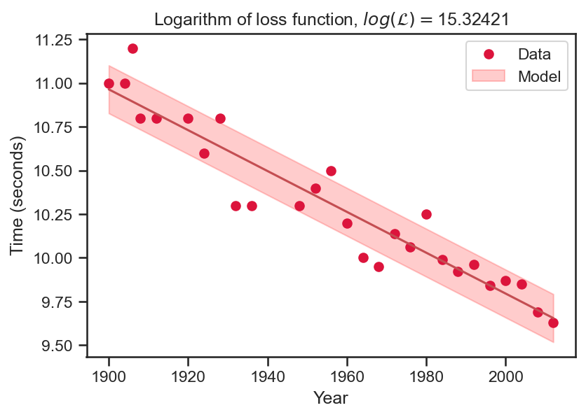
Visualizing the Gaussian noise model

Plot
Code

import pandas as pd
import numpy as np
import matplotlib.pyplot as plt
import seaborn as sns
sns.set(font_scale=1.0)
sns.set_style("white")
sns.set_style("ticks")
palette = sns.color_palette('deep')

df = pd.read_csv('notebooks/data/data100m.csv')
df.columns=['Year', 'Time']
N = df.shape[0]

max_year, min_year = df['Year'].values.max() , df['Year'].values.min()

x = (df['Year'].values.reshape(N,1) - min_year)/(max_year - min_year)
t = df['Time'].values.reshape(N,1)
X_func = lambda u : np.hstack([np.ones((u.shape[0],1)), u ])
X = X_func(x)
w_hat = np.linalg.inv(X.T @ X) @ X.T @ t
loss_func = 1./N * (t - X @ w_hat).T @ (t - X @ w_hat)

xgrid = np.linspace(0, 1, 100).reshape(100,1)
Xg = X_func(xgrid)
time_grid = Xg @ w_hat


xi = xgrid*(max_year - min_year) + min_year
xi = xi.flatten()
sigma_hat_squared = float( (1. / N) * (t.T @ t - t.T @ X @ w_hat) )
sigma_hat = np.sqrt(sigma_hat_squared)
yi = xi* 0 + sigma_hat

loss_func =  -N/2 * np.log(np.pi * 2)  - N * np.log(sigma_hat) - \
                   1./(2 * sigma_hat_squared) * np.sum((X @ w_hat - t)**2) 

fig = plt.figure(figsize=(6,4))
a, = plt.plot(df['Year'].values, df['Time'].values, 'o', color='crimson', label='Data')
plt.plot(xi, time_grid, '-', color='r')
c = plt.fill_between(xi, time_grid.flatten()-yi, time_grid.flatten()+yi, color='red', alpha=0.2, label='Model')
plt.xlabel('Year')
plt.ylabel('Time (seconds)')
loss_title = r'Logarithm of loss function, $log \left( \mathcal{L} \right)=$'+str(np.around(float(loss_func), 5))
plt.title(loss_title)
plt.legend([a,c], ['Data', 'Model'])
plt.savefig('olympics_last.png', dpi=150, bbox_inches='tight')
plt.close()

The graph on the left is the final model.

Lecture 6

The three model levels

Linear least squares model

Gaussian noise model (introducing the idea of likelihood)

Full Bayesian treatment (next time!)

Linear least squares

Linear least squares

Defining a good model

Linear least squares

Matrix-vector notation

Linear least squares

Minimizing the loss

Linear least squares

Linear least squares

Linear least squares

Linear least squares

With regularization

Maximum likelihood

Maximum likelihood

Defining the likelihood

Maximum likelihood

Defining the likelihood

Maximum likelihood

Maximizing the logarithm of the likelihood

Maximum likelihood

Maximizing the logarithm of the likelihood

Maximum likelihood

Maximizing the logarithm of the likelihood

Maximum likelihood

Visualizing the Gaussian noise model