Lecture 7

Towards Bayesian Inference

Gaussian noise model

• Recall, from last time, we had demonstrated that the maximum likelihood solution to the Gaussian noise model is equivalent to the least squares solution for the unknown weights, \mathbf{w}.

• Recall, that we had defined the likelihood as a function that describes how likely our data is, based on the model parameters.

• We shall now study the benefits of explicitly modelling noise:

  • quantifying uncertainty in the parameters;
  • expressing uncertainty in predictions.

Gaussian noise model

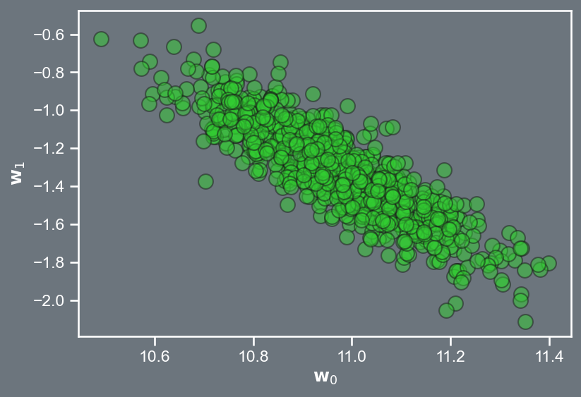
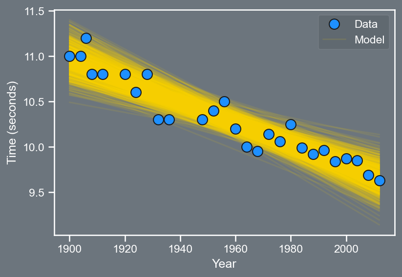
Consider a scenario where rather than solving \hat{\mathbf{w}} = \left( \mathbf{X}^{T} \mathbf{X} \right)^{-1} \mathbf{X}^{T} \mathbf{t} we randomly perturb \mathbf{t} and work out \hat{\mathbf{w}} for each perturbed value, i.e., \hat{\mathbf{w}}_{j} = \left( \mathbf{X}^{T} \mathbf{X} \right)^{-1} \mathbf{X}^{T} \left( \mathbf{t} + \boldsymbol{\epsilon}_{j} \right), \; \; \; \; \text{where} \; \; \boldsymbol{\epsilon}_{j} \sim \mathcal{N} \left( \mathbf{0}, \sigma^2 \mathbf{I} \right).

• Plot
• Code

import pandas as pd
import numpy as np
import matplotlib.pyplot as plt
import seaborn as sns
sns.set(font_scale=1.0)
sns.set_style("white")
sns.set_style("ticks")
palette = sns.color_palette('deep')
plt.style.use('dark_background')

df = pd.read_csv('notebooks/data/data100m.csv')
df.columns=['Year', 'Time']
N = df.shape[0]

max_year, min_year = df['Year'].values.max() , df['Year'].values.min()

x = (df['Year'].values.reshape(N,1) - min_year)/(max_year - min_year)
t = df['Time'].values.reshape(N,1)
X_func = lambda u : np.hstack([np.ones((u.shape[0],1)), u ])
X = X_func(x)

xgrid = np.linspace(0, 1, 100).reshape(100,1)
Xg = X_func(xgrid)
xi = xgrid*(max_year - min_year) + min_year
xi = xi.flatten()

# We will assume we 
sigma_hat = 0.4
M = 800
epsilon = np.random.randn(M, N) * sigma_hat
w_parameter = np.zeros((X.shape[1], M))
t_preds = np.zeros((100, M))

for j in range(0, M):
    epsilon_j = epsilon[j,:].reshape(N,1)
    t_j = t + epsilon_j
    w_j = np.linalg.inv(X.T @ X) @ X.T @ t_j
    w_parameter[:, j] = w_j.flatten()
    t_preds[:,j] = (Xg @ w_j).flatten()

# Plot 1
fig, ax = plt.subplots(figsize=(6,4))
fig.patch.set_facecolor('#6C757D')
ax.set_facecolor('#6C757D')
a, = plt.plot(w_parameter[0,:], w_parameter[1,:], 'o', color='limegreen', \
              label='Data', markeredgecolor='k', lw=1, ms=10, zorder=1, alpha=0.5)
plt.xlabel(r'$\mathbf{w}_0$')
plt.ylabel(r'$\mathbf{w}_1$')
plt.savefig('olympics_weights.png', dpi=150, bbox_inches='tight', facecolor="#6C757D")
plt.close()

# Plot 2
fig, ax = plt.subplots(figsize=(6,4))
fig.patch.set_facecolor('#6C757D')
ax.set_facecolor('#6C757D')
a, = plt.plot(df['Year'].values, df['Time'].values, 'o', color='dodgerblue', \
              label='Data', markeredgecolor='k', lw=1, ms=10, zorder=1)
c = plt.plot(xi, t_preds, '-', color='gold', alpha=0.1, zorder=0)
plt.xlabel('Year')
plt.ylabel('Time (seconds)')
plt.legend([a,c[0]], ['Data', 'Model'], framealpha=0.1)
plt.savefig('olympics_linear.png', dpi=150, bbox_inches='tight', facecolor="#6C757D")
plt.close()

:::

Gaussian noise model

It will be useful to understand how this change to the data—contaminated by noise—affects the model parameters. Recall, last time, we had expressed our model which was a product of univariate Gaussians as a single multivariate Gaussian of the form p \left( \mathbf{t} | \mathbf{X}, \mathbf{w}, \sigma^2 \right) = \mathcal{N}\left( \mathbf{Xw}, \sigma^2 \mathbf{I} \right)

In what follows, we would like to better describe the scatter we saw in the prior slide, by computing the mean and covariance of \mathbf{w}. Computing the expectation with respect to the generating distribution

\mathbb{E}_{p \left( \mathbf{t} | \mathbf{X}, \mathbf{w}, \sigma^2 \right)} \left[ \hat{\mathbf{w}} \right] = \int \hat{\mathbf{w}} p \left( \mathbf{t} | \mathbf{X}, \mathbf{w}, \sigma^2 \right) d \mathbf{t}

Substituting \mathbf{\hat{w}} = \left( \mathbf{X}^{T} \mathbf{X} \right)^{-1} \mathbf{X}^{T} \mathbf{t} into the expression above

\mathbb{E}_{p \left( \mathbf{t} | \mathbf{X}, \mathbf{w}, \sigma^2 \right)} \left[ \hat{\mathbf{w}} \right] = \left( \mathbf{X}^{T} \mathbf{X} \right)^{-1} \mathbf{X}^{T} \int \mathbf{t} p \left( \mathbf{t} | \mathbf{X}, \mathbf{w}, \sigma^2 \right) d \mathbf{t}

= \left( \mathbf{X}^{T} \mathbf{X} \right)^{-1} \mathbf{X}^{T} \mathbb{E}_{p \left( \mathbf{t} | \mathbf{X}, \mathbf{w}, \sigma^2 \right)} \left[ \mathbf{t} \right]

But since p \left( \mathbf{t} | \mathbf{X}, \mathbf{w}, \sigma^2 \right) = \mathcal{N}\left( \mathbf{Xw}, \sigma^2 \mathbf{I} \right), we can write \mathbb{E}_{p \left( \mathbf{t} | \mathbf{X}, \mathbf{w}, \sigma^2 \right)} \left[ \mathbf{t} \right] = \mathbf{Xw}.

Gaussian noise model

This yields

\mathbb{E}_{p \left( \mathbf{t} | \mathbf{X}, \mathbf{w}, \sigma^2 \right)} \left[ \hat{\mathbf{w}} \right] = \left( \mathbf{X}^{T} \mathbf{X} \right)^{-1} \mathbf{X}^{T} \mathbf{X w} = \mathbf{w}.

So, the expected value of our approximation \mathbf{\hat{w}} is the true parameter value \mathbf{w}. This means that our estimator is unbiased.

Any potential variability in \mathbf{\hat{w}} is captured by its covariance.

\begin{aligned} Cov \left[ \mathbf{\hat{w}} \right] & = \mathbb{E}_{p \left( \mathbf{t} | \mathbf{X}, \mathbf{w}, \sigma^2 \right)} \left[\mathbf{\hat{w}} \mathbf{\hat{w}}^{T} \right] - \mathbb{E}_{p \left( \mathbf{t} | \mathbf{X}, \mathbf{w}, \sigma^2 \right)} \left[ \mathbf{\hat{w}} \right] \mathbb{E}_{p \left( \mathbf{t} | \mathbf{X}, \mathbf{w}, \sigma^2 \right)} \left[ \mathbf{\hat{w}} \right]^{T} \\ & = \mathbb{E}_{p \left( \mathbf{t} | \mathbf{X}, \mathbf{w}, \sigma^2 \right)} \left[\mathbf{\hat{w}} \mathbf{\hat{w}}^{T} \right] - \mathbf{ww}^{T} \end{aligned} \tag{1}

Focusing solely on the first term, we have \begin{aligned} \mathbb{E}_{p \left( \mathbf{t} | \mathbf{X}, \mathbf{w}, \sigma^2 \right)} \left[\mathbf{\hat{w}} \mathbf{\hat{w}}^{T} \right] & = \mathbb{E}_{p \left( \mathbf{t} | \mathbf{X}, \mathbf{w}, \sigma^2 \right)} \left[ \left( \left(\mathbf{X}^{T} \mathbf{X} \right)^{-1} \mathbf{X}^{T} \mathbf{t} \right) \left( \left(\mathbf{X}^{T} \mathbf{X} \right)^{-1} \mathbf{X}^{T} \mathbf{t} \right)^{T} \right] \\ & = \left(\mathbf{X}^{T} \mathbf{X} \right)^{-1} \mathbf{X}^{T} \underbrace{\mathbb{E}_{p \left( \mathbf{t} | \mathbf{X}, \mathbf{w}, \sigma^2 \right)}\left[ \mathbf{tt}^{T} \right]}_{\text{need to determine}} \mathbf{X} \left( \mathbf{X}^{T} \mathbf{X} \right)^{-1} \end{aligned} \tag{2}

Gaussian noise model

To progress further, we recognize that by definition, the covariance of \mathbf{t} is \sigma^2 \mathbf{I}. Thus, we can write Cov \left[ \mathbf{t} \right] = \sigma^2 \mathbf{I} = \mathbb{E}_{p \left( \mathbf{t} | \mathbf{X}, \mathbf{w}, \sigma^2 \right)} \left[ \mathbf{tt}^{T} \right] - \mathbb{E}_{p \left( \mathbf{t} | \mathbf{X}, \mathbf{w}, \sigma^2 \right)} \left[ \mathbf{t} \right] \mathbb{E}_{p \left( \mathbf{t} | \mathbf{X}, \mathbf{w}, \sigma^2 \right)}\left[ \mathbf{t} \right]^{T}

Re-arranging this expression for the term in Equation 2 leads to \begin{aligned} \mathbb{E}_{p \left( \mathbf{t} | \mathbf{X}, \mathbf{w}, \sigma^2 \right)}\left[ \mathbf{tt}^{T} \right] & = \mathbb{E}_{p \left( \mathbf{t} | \mathbf{X}, \mathbf{w}, \sigma^2 \right)}\left[ \mathbf{t} \right] \mathbb{E}_{p \left( \mathbf{t} | \mathbf{X}, \mathbf{w}, \sigma^2 \right)}\left[ \mathbf{t} \right]^{T} + \sigma^2 \mathbf{I} \\ & = \mathbf{Xw} \left( \mathbf{Xw} \right)^{T} + \sigma^2 \mathbf{I} \\ & = \mathbf{Xww}^{T} \mathbf{X}^{T} + \sigma^2 \mathbf{I}. \end{aligned}

Substituting this expression into Equation 2:

\mathbb{E}_{p \left( \mathbf{t} | \mathbf{X}, \mathbf{w}, \sigma^2 \right)} \left[\mathbf{\hat{w}} \mathbf{\hat{w}}^{T} \right] = \left( \mathbf{X}^{T} \mathbf{X} \right)^{-1} \mathbf{X}^{T} \mathbf{X} \mathbf{w} \mathbf{w}^{T} \mathbf{X}^{T} \mathbf{X} \left( \mathbf{X}^{T} \mathbf{X} \right)^{-1} + \sigma^2 \left( \mathbf{X}^{T} \mathbf{X} \right)^{-1} \mathbf{X}^{T} \mathbf{X} \left( \mathbf{X}^{T} \mathbf{X} \right)^{-1} = \mathbf{ww}^{T} + \sigma^2 \left( \mathbf{X}^{T} \mathbf{X} \right)^{-1}

Gaussian noise model

Plugging this into Equation 1, we arrive at

\begin{aligned} Cov \left[ \mathbf{\hat{w}} \right] & = \mathbf{ww}^{T} + \sigma^2 \left( \mathbf{X}^{T} \mathbf{X} \right)^{-1} - \mathbf{ww}^{T} \\ & = \sigma^2 \left( \mathbf{X}^{T} \mathbf{X} \right)^{-1} \end{aligned}

The above matrix is important! Infact, you can show that Cov \left[ \mathbf{\hat{w}} \right] = - \left( \frac{\partial^2 \mathcal{L} }{\partial \mathbf{w} \partial \mathbf{w}^{T}} \right)^{-1}.

• This tells us that our confidence in the parameters is linked directly to the second derivative of the log-likelihood function.
• Low curvature corresponds to high uncertainty in \mathbf{\hat{w}}.
• We have an expression that tells us how much information about the parameter estimates \mathbf{\hat{w}}, our data gives us.

Gaussian noise model

• The matrix \sigma^2 \left( \mathbf{X}^{T} \mathbf{X} \right)^{-1} is the inverse of the Fisher Information matrix, \mathcal{I}, i.e., \mathcal{I} = \frac{1}{\sigma^2} \mathbf{X}^{T} \mathbf{X}.

• The elements of this matrix tell us how much information the data provides: the more negative the information value is, the more information there is.

• If the data is very noisy, the information content is lower.

Image source: Royal Society

Image link

Gaussian noise model

We have quantified the mean and covariance in the model parameters \mathbb{w}, but have not yet determined how they can be used to determine the mean and covariance of predicted times.

To aid this exposition, let us introduce \mathbf{X}_{new} \in \mathbb{R}^{S \times 2} where S is the number of new x locations (in this case time) at which our model needs to be evaluated, i.e., \mathbf{X}_{new}=\left[\begin{array}{cc} 1 & x^{new}_{1}\\ 1 & x^{new}_{2}\\ \vdots & \vdots\\ 1 & x^{new}_{S} \end{array}\right]

To predict \mathbf{t}_{new}, we simply multiply \mathbf{X}_{new} by the best set of model parameters \mathbf{\hat{w}}, i.e., \mathbf{t}_{new} = \mathbf{X}_{new} \mathbf{\hat{w}}

Using the formulas for the mean and covariance we can write \begin{aligned} \mathbb{E}_{p \left( \mathbf{t} | \mathbf{X}, \mathbf{w}, \sigma^2 \right)} \left[ \mathbf{t}_{new} \right] & = \mathbf{X}_{new} \mathbb{E}_{p \left( \mathbf{t} | \mathbf{X}, \mathbf{w}, \sigma^2 \right)} \left[ \mathbf{\hat{w}} \right] = \mathbf{X}_{new} \mathbf{w} \\ Cov_{p \left( \mathbf{t} | \mathbf{X}, \mathbf{w}, \sigma^2 \right)} \left[ \mathbf{t}_{new} \right] & = \sigma^2 \mathbf{X}^{T}_{new} \left( \mathbf{X}^{T} \mathbf{X} \right)^{-1} \mathbf{X}_{new} \\ & = \mathbf{X}_{new} Cov \left[ \mathbf{\hat{w}} \right] \mathbf{X}^{T}_{new} \end{aligned}

Gaussian noise model

• Plot
• Code

import pandas as pd
import numpy as np
import matplotlib.pyplot as plt
import seaborn as sns
sns.set(font_scale=1.0)
sns.set_style("white")
sns.set_style("ticks")
palette = sns.color_palette('deep')
plt.style.use('dark_background')

df = pd.read_csv('notebooks/data/data100m.csv')
df.columns=['Year', 'Time']
N = df.shape[0]

max_year, min_year = df['Year'].values.max() , df['Year'].values.min()

x = (df['Year'].values.reshape(N,1) - min_year)/(max_year - min_year)
t = df['Time'].values.reshape(N,1)
X_func = lambda u : np.hstack([np.ones((u.shape[0],1)), u ])
X = X_func(x)

xgrid = np.linspace(0, 1, 100).reshape(100,1)
Xg = X_func(xgrid)
xi = xgrid*(max_year - min_year) + min_year
xi = xi.flatten()

# We will assume we 
sigma_hat = 0.4
w_hat = np.linalg.inv(X.T @ X) @ X.T @ t
mean_t = (Xg @ w_hat).flatten()
cov_w = sigma_hat**2 * np.linalg.inv(X.T @ X)
cov_t = Xg @ cov_w @ Xg.T
std_t = np.sqrt(np.diag(cov_t)).flatten()

# Plot 1
fig, ax = plt.subplots(figsize=(6,4))
ax.set_facecolor('#6C757D')
fig.patch.set_facecolor('#6C757D')
a, = plt.plot(df['Year'].values, df['Time'].values, 'o', color='dodgerblue', \
              label='Data', markeredgecolor='k', lw=1, ms=10, zorder=1)
c = plt.plot(xi, t_preds, '-', color='gold', alpha=0.01, zorder=0)
c, = plt.plot(xi, mean_t, '-', color='red', zorder=3)

d = plt.fill_between(xi, mean_t -std_t, mean_t + std_t, color='crimson', alpha=0.3, zorder=4)
e = plt.fill_between(xi, mean_t - 2 * std_t, mean_t + 2 * std_t, color='crimson', alpha=0.1, zorder=5)

plt.xlabel('Year')
plt.ylabel('Time (seconds)')
plt.legend([a,c,d, e], ['Data', r'$\mathbb{E}[\mathbf{t}_new]$', r'$\sigma[\mathbf{t}_new]$', r'$2 \sigma[\mathbf{t}_new]$'], framealpha=0.1)
plt.savefig('olympics_uncertainty.png', dpi=150, bbox_inches='tight', facecolor="#6C757D")
plt.close()

Bayesian Model

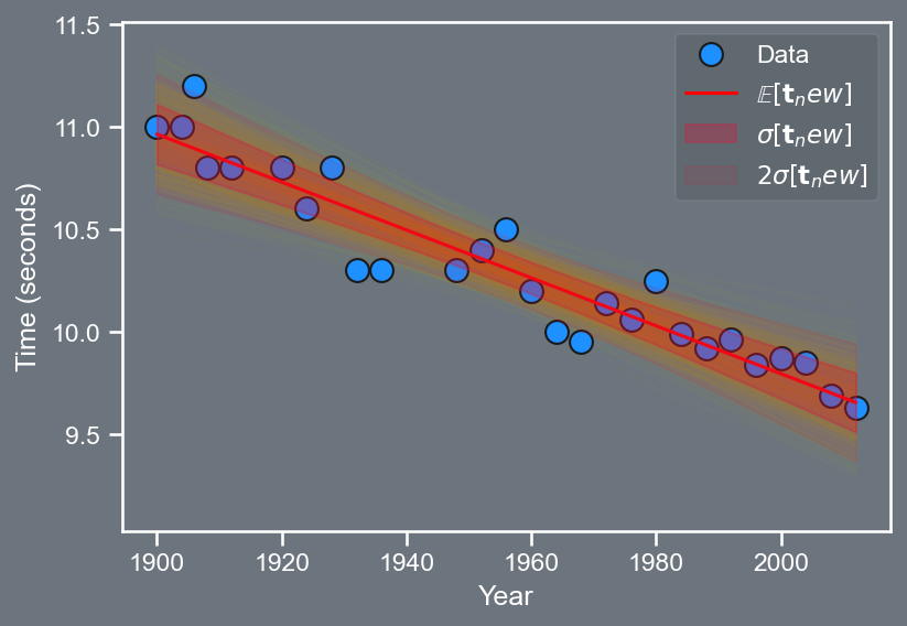
• Recall, earlier we had established that uncertainty in the model parameters \mathbf{\hat{w}} can be used to explain uncertainty in the data \mathbf{t}.

• We now introduce the notion of a prior to \mathbf{w}. To clarify, when introducing a prior to \mathbf{w}. For no better reason for now, we will assume a Gaussian distribution, i.e., p \left( \mathbf{w} | \boldsymbol{\mu}_{0}, \boldsymbol{\Sigma}_{0} \right) = \mathcal{N} \left( \boldsymbol{\mu}_{0}, \boldsymbol{\Sigma}_{0} \right) where the choice of the mean \boldsymbol{\mu}_{0} and covariance \boldsymbol{\Sigma}_{0} is typically selected by the user / practitioner.

• From a notation standpoint, note that we will not explicitly condition on \boldsymbol{\mu}_{0} and \boldsymbol{\Sigma}_{0}, i.e., we will use p \left( \mathbf{w} | \mathbf{t}, \mathbf{X}, \sigma^2 \right) instead of p \left( \mathbf{w} | \mathbf{t}, \mathbf{X}, \sigma^2, \boldsymbol{\mu}_{0}, \boldsymbol{\Sigma}_{0} \right).

Scatter in the model parameters, \mathbf{w}.

Bayesian Model

• The likelihood, p \left( \mathbf{t} | \mathbf{w}, \mathbf{X}, \sigma^2 \right) is the quantity that we had maximized before.

• Note that our model is of the form \mathbf{t} = \mathbf{Xw} + \boldsymbol{\epsilon}, where \boldsymbol{\epsilon} \sim \mathcal{N}\left(\mathbf{0}, \sigma^2 \mathbf{I} \right).

• As we have shown before, a Gaussian random variable plus a constant is equivalent to a Gaussian random variable with a shifted mean, i.e., p \left( \mathbf{t} | \mathbf{w}, \mathbf{X}, \sigma^2 \right) = \mathcal{N}\left( \mathbf{Xw}, \sigma^2 \mathbf{I} \right)

• The likelihood is sometimes called the noise model.

Bayesian Model

• Notionally, we can express the posterior density as \textsf{posterior} \propto \textsf{likelihood} \times \textsf{prior} where the symbol \propto hides the proportionality factor given by \int \text{likelihood} \times \text{prior}, where the integral is evaluated over the space of prior.

• This proportionality factor is also known as the:

  • marginal likelihood
  • evidence
  • prior predictive
  • partition function.

• The posterior is written using Bayes’ rule via p \left( \mathbf{w} | \mathbf{t}, \mathbf{X}, \sigma^2 \right) = \frac{p \left( \mathbf{t} | \mathbf{w}, \mathbf{X}, \sigma^2 \right) p \left( \mathbf{w} \right) }{\int p \left( \mathbf{t} | \mathbf{w}, \mathbf{X}, \sigma^2 \right) p \left( \mathbf{w} \right) d\mathbf{w} } = \frac{p \left( \mathbf{t} | \mathbf{w}, \mathbf{X}, \sigma^2 \right) p \left( \mathbf{w} \right) }{p \left( \mathbf{t} | \mathbf{X}, \sigma^2 \right)}

Bayesian Model

Prior

p \left( \mathbf{w} \right)

Likelihood

p \left( \mathbf{t} | \mathbf{w}, \mathbf{X}, \sigma^2 \right)

Posterior

p \left( \mathbf{w} | \mathbf{t}, \mathbf{X}, \sigma^2 \right)

where

• \mathbf{X} encodes the model attributes (or inputs or covariates),
• \mathbf{t} are the observed values (or outputs), and
• \sigma^2 in this case is an assumed noise.

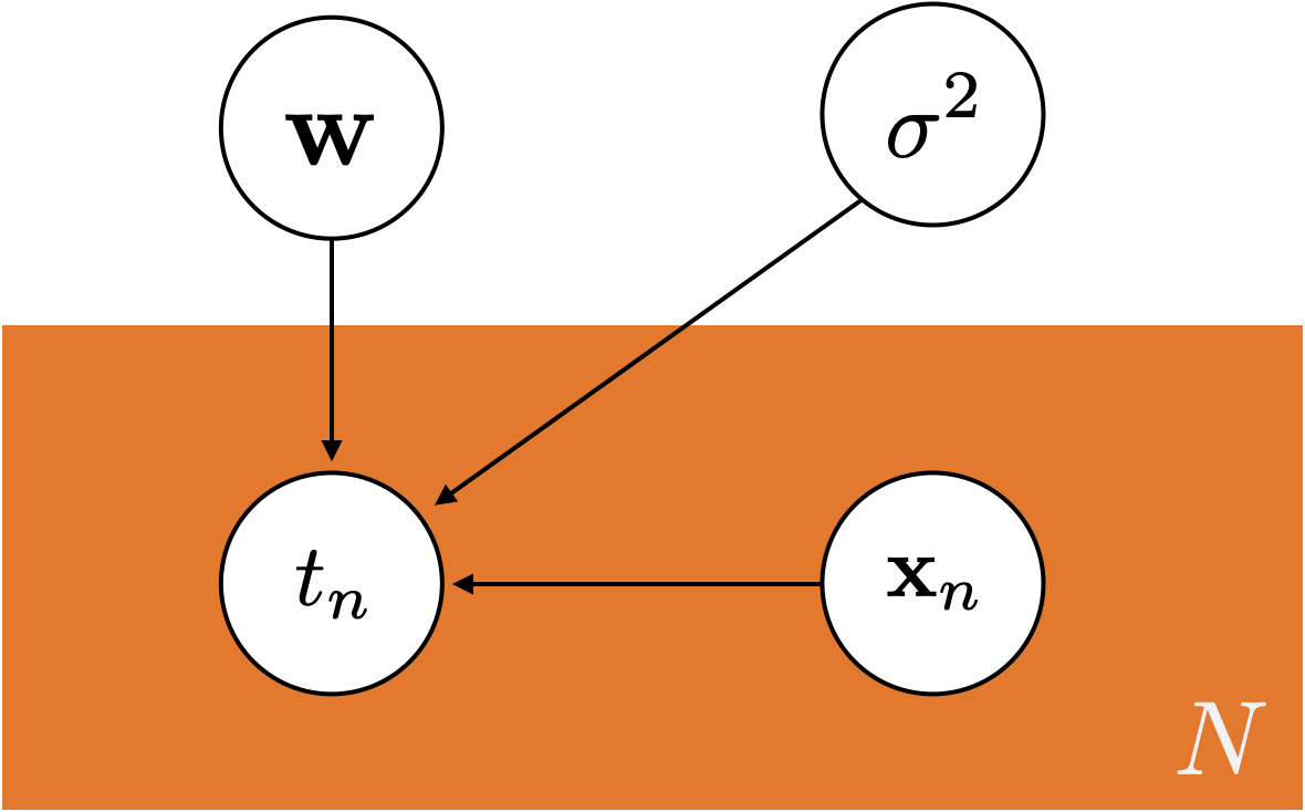
A graphical representation of the model.

Bayesian Model

• We shall now solve for this posterior, assuming that both the prior and likelihood are Gaussian.

• In this case, we know that the posterior will be Gaussian!

p \left( \mathbf{w} | \mathbf{t}, \mathbf{X}, \sigma^2 \right) \propto p \left( \mathbf{t} | \mathbf{w}, \mathbf{X}, \sigma^2 \right) p \left( \mathbf{w} \right) \begin{aligned} = \frac{1}{\left( 2 \pi \right)^{N/2} | \sigma^2 \mathbf{I} |^{1/2} } exp \left( - \frac{1}{2} \left( \mathbf{t} - \mathbf{Xw} \right)^{T} \left( \sigma^2 \mathbf{I} \right)^{-1} \left( \mathbf{t} - \mathbf{Xw} \right) \right) \\ \times \frac{1}{\left( 2 \pi \right)^{N/2} | \boldsymbol{\Sigma}_{0} |^{1/2} } exp \left( - \frac{1}{2} \left( \mathbf{w} - \boldsymbol{\mu}_{0} \right)^{T} \boldsymbol{\Sigma}_{0}^{-1} \left( \mathbf{w} - \boldsymbol{\mu}_{0} \right) \right) \end{aligned} \propto exp \left( - \frac{1}{2} \left( \mathbf{t} - \mathbf{Xw} \right)^{T} \left( \sigma^2 \mathbf{I} \right)^{-1} \left( \mathbf{t} - \mathbf{Xw} \right) \right) \times exp \left( - \frac{1}{2} \left( \mathbf{w} - \boldsymbol{\mu}_{0} \right)^{T} \boldsymbol{\Sigma}_{0}^{-1} \left( \mathbf{w} - \boldsymbol{\mu}_{0} \right) \right)

• Try and work through this derivation; we shall continue next time from here.