Lecture 8

Bayesian Inference

Bayesian model

Deriving the posterior

Recall, from Lecture 8

p \left( \mathbf{w} | \mathbf{t}, \mathbf{X}, \sigma^2 \right) \propto p \left( \mathbf{t} | \mathbf{w}, \mathbf{X}, \sigma^2 \right) p \left( \mathbf{w} \right) \begin{aligned} = \frac{1}{\left( 2 \pi \right)^{N/2} | \sigma^2 \mathbf{I} |^{1/2} } exp \left( - \frac{1}{2} \left( \mathbf{t} - \mathbf{Xw} \right)^{T} \left( \sigma^2 \mathbf{I} \right)^{-1} \left( \mathbf{t} - \mathbf{Xw} \right) \right) \\ \times \frac{1}{\left( 2 \pi \right)^{N/2} | \boldsymbol{\Sigma}_{0} |^{1/2} } exp \left( - \frac{1}{2} \left( \mathbf{w} - \boldsymbol{\mu}_{0} \right)^{T} \boldsymbol{\Sigma}_{0}^{-1} \left( \mathbf{w} - \boldsymbol{\mu}_{0} \right) \right) \end{aligned} \propto exp \left( - \frac{1}{2} \left( \mathbf{t} - \mathbf{Xw} \right)^{T} \left( \sigma^2 \mathbf{I} \right)^{-1} \left( \mathbf{t} - \mathbf{Xw} \right) \right) \times exp \left( - \frac{1}{2} \left( \mathbf{w} - \boldsymbol{\mu}_{0} \right)^{T} \boldsymbol{\Sigma}_{0}^{-1} \left( \mathbf{w} - \boldsymbol{\mu}_{0} \right) \right)

We shall now continue this derivation.

Bayesian model

Deriving the posterior

p \left( \mathbf{w} | \mathbf{t}, \mathbf{X}, \sigma^2 \right) \propto exp \left\{ - \frac{1}{2} \left( \frac{1}{\sigma^2} \left( \mathbf{t} - \mathbf{Xw} \right)^{T} \left( \mathbf{t} - \mathbf{Xw} \right) + \left( \mathbf{w} - \boldsymbol{\mu}_{0} \right)^{T} \boldsymbol{\Sigma }_{0}^{-1} \left( \mathbf{w} - \boldsymbol{\mu}_{0} \right) \right) \right\}

Multiplying the terms in the bracket out, and removing any terms that do not involve a \mathbf{w} yields

\begin{aligned} p \left( \mathbf{w} | \mathbf{t}, \mathbf{X}, \sigma^2 \right) & \propto \\ & exp \left\{ - \frac{1}{2} \left( - \frac{2}{\sigma^2} \mathbf{t}^{T} \mathbf{Xw} + \frac{1}{\sigma^2} \mathbf{w}^{T} \mathbf{X}^{T}\mathbf{X} \mathbf{w} + \mathbf{w}^{T} \boldsymbol{\Sigma}_{0}^{-1} \mathbf{w} - 2 \boldsymbol{\mu}_{0}^{T} \boldsymbol{\Sigma}_{0}^{-1}\mathbf{w} \right) \right\} \end{aligned} \tag{1}

The trick is to recognize that since our posterior is Gaussian, it must have the form

\begin{aligned} p \left( \mathbf{w} | \mathbf{t}, \mathbf{X}, \sigma^2 \right) = \mathcal{N}\left(\boldsymbol{\mu}_{\mathbf{w}}, \boldsymbol{\Sigma}_{\mathbf{w}} \right) \end{aligned} \tag{2}

Bayesian model

Deriving the posterior

If we expand Equation 2, we arrive at

\begin{aligned} p \left( \mathbf{w} | \mathbf{t}, \mathbf{X}, \sigma^2 \right) & \propto exp \left\{ - \frac{1}{2} \left( \mathbf{w} - \boldsymbol{\mu}_{\mathbf{w}} \right)^{T} \boldsymbol{\Sigma}_{\mathbf{w}}^{-1} \left( \mathbf{w} - \boldsymbol{\mu}_{\mathbf{w}} \right) \right\} \\ & \propto exp \left\{ - \frac{1}{2} \left( \mathbf{w}^{T} \boldsymbol{\Sigma}^{-1}_{\mathbf{w}} \mathbf{w} - 2 \boldsymbol{\mu}_{\mathbf{w}}^{T} \boldsymbol{\Sigma}_{\mathbf{w}}^{-1} \mathbf{w} \right) \right\} \end{aligned} \tag{3}

The quadratic terms in \mathbf{w} in Equation 3 must match those we had in Equation 1. Thus we can write \begin{aligned} \mathbf{w}^{T} \boldsymbol{\Sigma}_{\mathbf{w}}^{-1} \mathbf{w} & = \frac{1}{\sigma^2} \mathbf{w}^{T} \mathbf{X}^{T} \mathbf{X} \mathbf{w} + \mathbf{w}^{T} \boldsymbol{\Sigma}_{0}^{-1} \mathbf{w} \\ & = \mathbf{w}^{T} \left( \frac{1}{\sigma^2} \mathbf{X}^{T} \mathbf{X} + \boldsymbol{\Sigma}_{0}^{-1} \right) \mathbf{w} \end{aligned}

As for the expectation, we equate the linear terms in Equation 1 with those in Equation 3 \begin{aligned} -2 \boldsymbol{\mu}_{\mathbf{w}}^{T} \boldsymbol{\Sigma}_{\mathbf{w}}^{-1}\mathbf{w} = - \frac{2}{\sigma^2} \mathbf{t}^{T} \mathbf{Xw} - 2 \boldsymbol{\mu}_{0}^{T} \boldsymbol{\Sigma}_{0}^{-1} \mathbf{w} \end{aligned}

Bayesian model

Deriving the posterior

Continuing this expansion

\begin{aligned} \boldsymbol{\mu}_{\mathbf{w}}^{T} \boldsymbol{\Sigma}_{\mathbf{w}}^{-1} & = \frac{1}{\sigma^2} \mathbf{t}^{T} \mathbf{X} + \boldsymbol{\mu}_{0}^{T} \boldsymbol{\Sigma}_{0}^{-1} \\ \boldsymbol{\mu}_{\mathbf{w}}^{T} & = \left( \frac{1}{\sigma^2} \mathbf{t}^{T} \mathbf{X} + \boldsymbol{\mu}_{0}^{T} \boldsymbol{\Sigma}_{0}^{-1} \right) \boldsymbol{\Sigma}_{\mathbf{w}} \\ \Rightarrow \boldsymbol{\mu}_{\mathbf{w}} & = \mathbf{\Sigma}_{\mathbf{w}} \left( \frac{1}{\sigma^2} \mathbf{X}^{T} \mathbf{t} + \boldsymbol{\Sigma}^{-1}_{0} \boldsymbol{\mu}_{0} \right) \end{aligned}

where the last statement is due to \boldsymbol{\Sigma}_{\mathbf{w}} = \boldsymbol{\Sigma}_{\mathbf{w}}^{T}, i.e., the covariance matrix is symmetric.

To summarize, we have now worked out our posterior

p \left( \mathbf{w} | \mathbf{t}, \mathbf{X}, \sigma^2 \right) = \mathcal{N}\left( \boldsymbol{\mu}_{\mathbf{w}}, \boldsymbol{\Sigma}_{\mathbf{w}} \right) where \boldsymbol{\mu}_{\mathbf{w}} = \mathbf{\Sigma}_{\mathbf{w}} \left( \frac{1}{\sigma^2} \mathbf{X}^{T} \mathbf{t} + \boldsymbol{\Sigma}^{-1}_{0} \boldsymbol{\mu}_{0} \right) \; \; \text{and} \; \; \boldsymbol{\Sigma}_{\mathbf{w}} = \left( \frac{1}{\sigma^2} \mathbf{X}^{T} \mathbf{X} + \boldsymbol{\Sigma}_{0}^{-1} \right)^{-1}

Bayesian model

Maximum a posteriori estimate

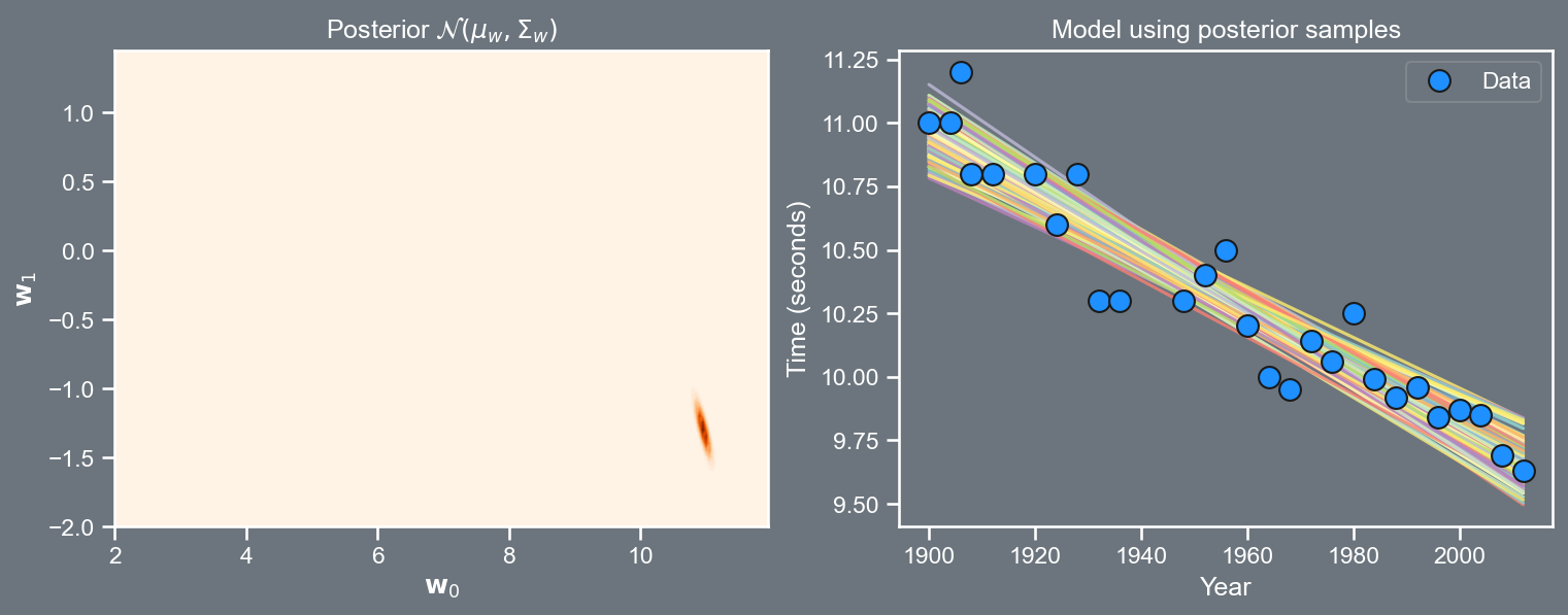
If we set the prior mean to be zero, i.e., \boldsymbol{\mu}_{0} = \left[ 0, 0, \ldots, 0 \right]^{T}, the resulting value of \boldsymbol{\mu}_{\mathbf{w}} looks very similar to the maximum likelihood solution from before.
Note, that because the posterior p \left( \mathbf{w} | \mathbf{t}, \mathbf{X}, \sigma^2 \right) is Gaussian, the most likely value of \mathbf{w} is the mean of the posterior, \boldsymbol{\mu}_{\mathbf{w}}. .
This is known as the maximum a posteriori (MAP) estimate of \mathbf{w} and can also be thought of as the maximum value of the joint density p \left( \mathbf{w}, \mathbf{t} | \mathbf{X} \sigma^2, \boldsymbol{\mu}_{0}, \boldsymbol{\Sigma}_{0} \right) (which is the likelihood \times prior).

Bayesian model

Predictive density

Just as we did last time, it will be useful to make predictions. To do this, we once again use \mathbf{X}_{new} \in \mathbb{R}^{S \times 2} where S is the number of new x locations (in this case time) at which our model needs to be evaluated, i.e., \mathbf{X}_{new}=\left[\begin{array}{cc} 1 & x^{new}_{1}\\ 1 & x^{new}_{2}\\ \vdots & \vdots\\ 1 & x^{new}_{S} \end{array}\right]

We are interested in the predictive density

p \left( \mathbf{t}_{new} | \mathbf{X}_{new}, \mathbf{X}, \mathbf{t}, \sigma^2 \right)

Notice, that this density is not conditioned on \mathbf{w}. We are going to integrate out \mathbf{w} by taking an expectation with respect to the posterior p \left( \mathbf{w} | \mathbf{t}, \mathbf{X}, \sigma^2 \right), i.e.,

\begin{aligned} p \left( \mathbf{t}_{new} | \mathbf{X}_{new}, \mathbf{X}, \mathbf{t}, \sigma^2 \right) & = \mathbb{E}_{p \left( \mathbf{w} | \mathbf{t}, \mathbf{X}, \sigma^2 \right)} \left[ p \left( \mathbf{t}_{new} | \mathbf{w}, \mathbf{X}_{new}, \sigma^2 \right)\right] \\ & = \int p \left( \mathbf{t}_{new} | \mathbf{w}, \mathbf{X}_{new}, \sigma^2 \right) p \left( \mathbf{w} | \mathbf{t}, \mathbf{X}, \sigma^2 \right) d\mathbf{w} \end{aligned}

Bayesian model

Predictive density

This leads to the predictive density form given by p \left( \mathbf{t}_{new} | \mathbf{X}_{new}, \mathbf{X}, \mathbf{t}, \sigma^2 \right) = \mathcal{N} \left( \mathbf{X}_{new} \boldsymbol{\mu}_{\mathbf{w}} , \sigma^2 \mathbf{I} + \mathbf{X}_{new}^{T} \boldsymbol{\Sigma}_{\mathbf{w}} \mathbf{X}_{new} \right) \tag{4}
Try proving this yourself! You may find section 2.3.2 of Bishop useful
The inclusion of the \sigma^2 \mathbf{I} term is optional, i.e., if we wish to replicate the true signal (without noise) this can be negated. However, if we wish to model the realistic data generation process then the noise should be incorporated.

Bayesian model

import pandas as pd
import numpy as np
import matplotlib
import matplotlib.pyplot as plt
from scipy.stats import multivariate_normal
import seaborn as sns
sns.set(font_scale=1.0)
sns.set_style("white")
sns.set_style("ticks")
palette = sns.color_palette('deep')
plt.style.use('dark_background')
df = pd.read_csv('notebook/data/data100m.csv')
df.columns=['Year', 'Time']
N = df.shape[0]

# Data & basis
max_year, min_year = df['Year'].values.max() , df['Year'].values.min()
x = (df['Year'].values.reshape(N,1) - min_year)/(max_year - min_year)
t = df['Time'].values.reshape(N,1)
X_func = lambda u : np.hstack([np.ones((u.shape[0],1)), u ])
X = X_func(x)

# For prediction / plotting
xgrid = np.linspace(0, 1, 100).reshape(100,1)
Xg = X_func(xgrid)
xi = xgrid*(max_year - min_year) + min_year
xi = xi.flatten()
sigma_hat = 0.2
sigma_w = 2.0

# Prior
mu_0 = np.array([[7],
                 [0]])
Sigma_0 = np.array([[5.0, -0.8],
                    [-0.8, 0.5]])
inv_Sigma_0 = np.eye(X.shape[1]) * 1/(sigma_w**2)
prior = multivariate_normal(mu_0.flatten(), Sigma_0)

# Posterior
Sigma_w = np.linalg.inv(1./(sigma_hat**2) * (X.T @ X) + inv_Sigma_0)
mu_w = Sigma_w @ (1./(sigma_hat**2) * (X.T @ t) + (inv_Sigma_0 @ mu_0) )
posterior = multivariate_normal(mu_w.flatten(), Sigma_w)

# Plotting support
ww1, ww2 = np.mgrid[2:12:.05, -2:1.5:.05]
pos = np.dstack((ww1, ww2))

fig, ax = plt.subplots(2, figsize=(12,4))
fig.patch.set_facecolor('#6C757D')
ax[0].set_fc('#6C757D')
plt.subplot(121)
plt.contourf(ww1, ww2, prior.pdf(pos), 30, cmap=plt.cm.Oranges)
plt.title(r'Prior $\mathcal{N}(\mu_0, \Sigma_0)$')
plt.xlabel(r'$\mathbf{w}_0$')
plt.ylabel(r'$\mathbf{w}_1$')
fig.patch.set_facecolor('#6C757D')

plt.subplot(122)
plt.rcParams['axes.facecolor']='#6C757D'
ax[1].set_facecolor('#6C757D')
random_samples = 200
plt.plot(xi, Xg @ prior.rvs(random_samples).T, alpha=0.7)
plt.xlabel('Year')
plt.title('model using prior samples')
plt.ylabel('Time (seconds)')
plt.savefig('prior.png', dpi=150, bbox_inches='tight', facecolor="#6C757D")
plt.close()

Bayesian model

Visualizing the posterior

Plot
Code

import pandas as pd
import numpy as np
import matplotlib
import matplotlib.pyplot as plt
from scipy.stats import multivariate_normal
import seaborn as sns
sns.set(font_scale=1.0)
sns.set_style("white")
sns.set_style("ticks")
palette = sns.color_palette('deep')
plt.style.use('dark_background')
df = pd.read_csv('notebook/data/data100m.csv')
df.columns=['Year', 'Time']
N = df.shape[0]

# Data & basis
max_year, min_year = df['Year'].values.max() , df['Year'].values.min()
x = (df['Year'].values.reshape(N,1) - min_year)/(max_year - min_year)
t = df['Time'].values.reshape(N,1)
X_func = lambda u : np.hstack([np.ones((u.shape[0],1)), u ])
X = X_func(x)

# For prediction / plotting
xgrid = np.linspace(0, 1, 100).reshape(100,1)
Xg = X_func(xgrid)
xi = xgrid*(max_year - min_year) + min_year
xi = xi.flatten()
sigma_hat = 0.2
sigma_w = 2.0

# Prior
mu_0 = np.array([[7],
                 [0]])
Sigma_0 = np.array([[5.0, -0.8],
                    [-0.8, 0.5]])
inv_Sigma_0 = np.eye(X.shape[1]) * 1/(sigma_w**2)
prior = multivariate_normal(mu_0.flatten(), Sigma_0)

# Posterior
Sigma_w = np.linalg.inv(1./(sigma_hat**2) * (X.T @ X) + inv_Sigma_0)
mu_w = Sigma_w @ (1./(sigma_hat**2) * (X.T @ t) + (inv_Sigma_0 @ mu_0) )
posterior = multivariate_normal(mu_w.flatten(), Sigma_w)

# Plotting support
ww1, ww2 = np.mgrid[2:12:.05, -2:1.5:.05]
pos = np.dstack((ww1, ww2))

fig, ax = plt.subplots(2, figsize=(12,4))
fig.patch.set_facecolor('#6C757D')
ax[0].set_fc('#6C757D')
plt.subplot(121)
plt.contourf(ww1, ww2, posterior.pdf(pos), 30, cmap=plt.cm.Oranges)
plt.title(r'Posterior $\mathcal{N}(\mu_w, \Sigma_w)$')
plt.xlabel(r'$\mathbf{w}_0$')
plt.ylabel(r'$\mathbf{w}_1$')
fig.patch.set_facecolor('#6C757D')

plt.subplot(122)
plt.rcParams['axes.facecolor']='#6C757D'
ax[1].set_facecolor('#6C757D')
plt.plot(xi, Xg @ posterior.rvs(random_samples).T, zorder=-1, alpha=0.8)
a, = plt.plot(df['Year'].values, df['Time'].values, 'o', color='dodgerblue', \
              label='Data', markeredgecolor='k', lw=1, ms=10, zorder=1)
plt.xlabel('Year')
plt.title('model using posterior samples')
plt.legend([a ], ['Data'], framealpha=0.2)
plt.ylabel('Time (seconds)')
plt.savefig('posterior.png', dpi=150, bbox_inches='tight', facecolor="#6C757D")
plt.show()
plt.close()

Bayesian model

Conjugacy

A likelihood-prior pair is said to be conjugate if they result in a posterior which is of the same form as the prior.
This enables us to compute the posterior density analytically (as we have done) without having to worry about the marginal likelihood (the denominator in Bayes’ rule).
Some commonly used prior and likelihood distributions are given below.

Prior	Likelihood
Gaussian	Gaussian
Beta	Binomial
Gamma	Gaussian
Dirichlet	Multinomial

Bayesian model

Marginal likelihood re-visited

The marginal likelihood for a Bayesian model is given by \text{marginal likelihood} = \int \text{likelihood} \times \text{prior} \; d \mathbf{w}
The marginal likelihood for our Gaussian prior and Gaussian likelihood model is given by \begin{aligned} p \left( \mathbf{t} | \mathbf{X}, \boldsymbol{\mu}_{0}, \boldsymbol{\Sigma}_{0} \right) & = \int p \left( \mathbf{t} | \mathbf{X}, \mathbf{w}, \sigma^2 \right) p \left( \mathbf{w} | \boldsymbol{\mu}_{0} , \boldsymbol{\Sigma}_{0} \right) d \mathbf{w} \\ & = \mathcal{N} \left( \mathbf{X} \boldsymbol{\mu}_{0}, \sigma^2 \mathbf{I}_{N} + \mathbf{X} \boldsymbol{\Sigma}_{0} \mathbf{X}^{T} \right) \end{aligned}
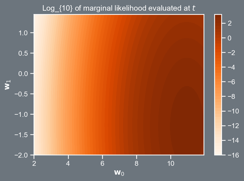
Note that it has the same form as Equation 4, and it is evaluated at \mathbf{t}, i.e., the observed winning times.

Bayesian model

Marginal likelihood re-visited

Plot
Code

The plot on the right shows the logarithm of the marginal likelihood.
Note that where the contours peak corresponds to values of \mathbf{w} that better explain the data \mathbf{t}, given its uncertainty \sigma^2, and the model as encoded into \mathbf{X}.

import pandas as pd
import numpy as np
import matplotlib
import matplotlib.pyplot as plt
from scipy.stats import multivariate_normal
import seaborn as sns
sns.set(font_scale=1.0)
sns.set_style("white")
sns.set_style("ticks")
palette = sns.color_palette('deep')
plt.style.use('dark_background')
df = pd.read_csv('notebook/data/data100m.csv')
df.columns=['Year', 'Time']
N = df.shape[0]

# Data & basis
max_year, min_year = df['Year'].values.max() , df['Year'].values.min()
x = (df['Year'].values.reshape(N,1) - min_year)/(max_year - min_year)
t = df['Time'].values.reshape(N,1)
X_func = lambda u : np.hstack([np.ones((u.shape[0],1)), u ])
X = X_func(x)

# For prediction / plotting
xgrid = np.linspace(0, 1, 100).reshape(100,1)
Xg = X_func(xgrid)
xi = xgrid*(max_year - min_year) + min_year
xi = xi.flatten()
sigma_hat = 0.2
sigma_w = 2.0

# Prior
mu_0 = np.array([[7],
                 [0]])
Sigma_0 = np.array([[5.0, -0.8],
                    [-0.8, 0.5]])
inv_Sigma_0 = np.eye(X.shape[1]) * 1/(sigma_w**2)
prior = multivariate_normal(mu_0.flatten(), Sigma_0)

# Posterior
Sigma_w = np.linalg.inv(1./(sigma_hat**2) * (X.T @ X) + inv_Sigma_0)
mu_w = Sigma_w @ (1./(sigma_hat**2) * (X.T @ t) + (inv_Sigma_0 @ mu_0) )
posterior = multivariate_normal(mu_w.flatten(), Sigma_w)

# Plotting support
ww1, ww2 = np.mgrid[2:12:.05, -2:1.5:.05]
pos = np.dstack((ww1, ww2))

marginal_like_val = np.ones((ww1.shape[0], ww1.shape[1]))

for i in range(0, ww1.shape[0]):
    for j in range(0, ww1.shape[1]):
        mu_0 = np.array([ ww1[i,j], ww2[i,j] ]).reshape(2, 1)
        marginal_likelihood_dist = multivariate_normal( (X @ mu_0).flatten(), \
                                               sigma_hat**2 * np.eye(t.shape[0]) + X @ X.T)
        marginal_like_val[i, j] = marginal_likelihood_dist.pdf(t.flatten())

fig, ax = plt.subplots(figsize=(6,4))
fig.patch.set_facecolor('#6C757D')
ax.set_fc('#6C757D')
c = plt.contourf(ww1, ww2, np.log10(marginal_like_val), 60, cmap=plt.cm.Oranges)
plt.colorbar(c)
plt.title(r'Log_{10} of marginal likelihood evaluated at $t$')
plt.xlabel(r'$\mathbf{w}_0$')
plt.ylabel(r'$\mathbf{w}_1$')
plt.savefig('marginal_log.png', dpi=150, bbox_inches='tight', facecolor="#6C757D")
plt.close()

Bayesian model

A function space perspective

Sampling \mathbf{t} conditioned on \mathbf{w} vs. sampling \mathbf{t} directly from the marginal likelihood are statistically equivalent.
Removing \mathbf{w} from our model (effectively making it non-parametric) opens the door to thinking of priors in the space of functions, and not just in the space of model parameters.
This is arguably one of the main ideas in Gaussian processes, that I will introduce next time we meet.