import pandas as pd
import numpy as np
import matplotlib
import matplotlib.pyplot as plt
from scipy.stats import multivariate_normal
from scipy.linalg import cholesky, solve_triangular
import seaborn as sns
sns.set(font_scale=1.0)
sns.set_style("white")
sns.set_style("ticks")
palette = sns.color_palette('deep')
plt.style.use('dark_background')
def kernel(xa, xb, amp, ll):
Xa, Xb = get_tiled(xa, xb)
return amp**2 * np.exp(-0.5 * 1./ll**2 * (Xa - Xb)**2 )
def get_tiled(xa, xb):
m, n = len(xa), len(xb)
xa, xb = xa.reshape(m,1) , xb.reshape(n,1)
Xa = np.tile(xa, (1, n))
Xb = np.tile(xb.T, (m, 1))
return Xa, Xb
X = np.linspace(-2, 2, 150)
cov_1 = kernel(X, X, 1, 0.1)
mu_1 = np.zeros((150,))
prior_1 = multivariate_normal(mu_1, cov_1, allow_singular=True)
cov_2 = kernel(X, X, 0.5, 1)
mu_2 = np.zeros((150,))
prior_2 = multivariate_normal(mu_2, cov_2, allow_singular=True)
random_samples = 50
fig, ax = plt.subplots(2, figsize=(12,4))
fig.patch.set_facecolor('#6C757D')
ax[0].set_fc('#6C757D')
plt.subplot(121)
plt.plot(X, prior_1.rvs(random_samples).T, alpha=0.5)
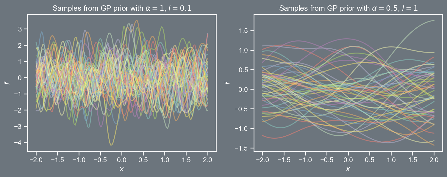
plt.title(r'Samples from GP prior with $\alpha=1$, $l=0.1$')
plt.xlabel(r'$x$')
plt.ylabel(r'$f$')
#plt.ylabel(r'$\mathbf{w}_1$')
fig.patch.set_facecolor('#6C757D')
plt.subplot(122)
plt.rcParams['axes.facecolor']='#6C757D'
ax[1].set_facecolor('#6C757D')
plt.plot(X, prior_2.rvs(random_samples).T, alpha=0.5)
plt.title(r'Samples from GP prior with $\alpha=0.5$, $l=1$')
plt.xlabel(r'$x$')
plt.ylabel(r'$f$')
plt.savefig('prior.png', dpi=150, bbox_inches='tight', facecolor="#6C757D")
plt.close()Lecture 9
An Introduction to Gaussian Processes
An introduction to Gaussian processes
Visualizing GP priors
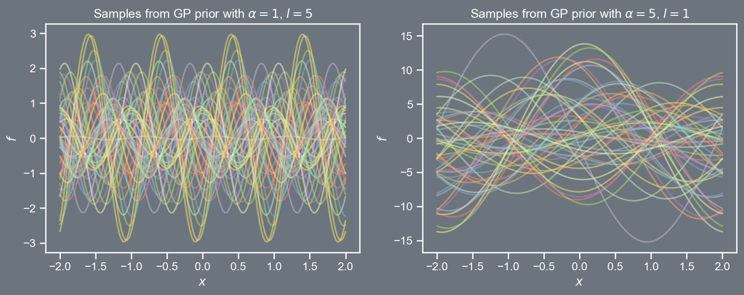
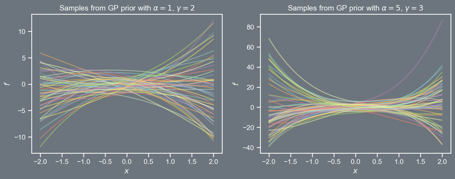
Defining a grid of points \mathcal{X} \equiv \left[-2, 2 \right], and choosing values for \alpha and l, we can sample vectors \mathbf{t} from the GP prior \mathcal{N}\left(\mathbf{0}, \mathbf{C} \right), where \mathbf{C}_{ij} = k \left( \boldsymbol{x}_{i}, \boldsymbol{x}_{j} \right).
An introduction to Gaussian processes
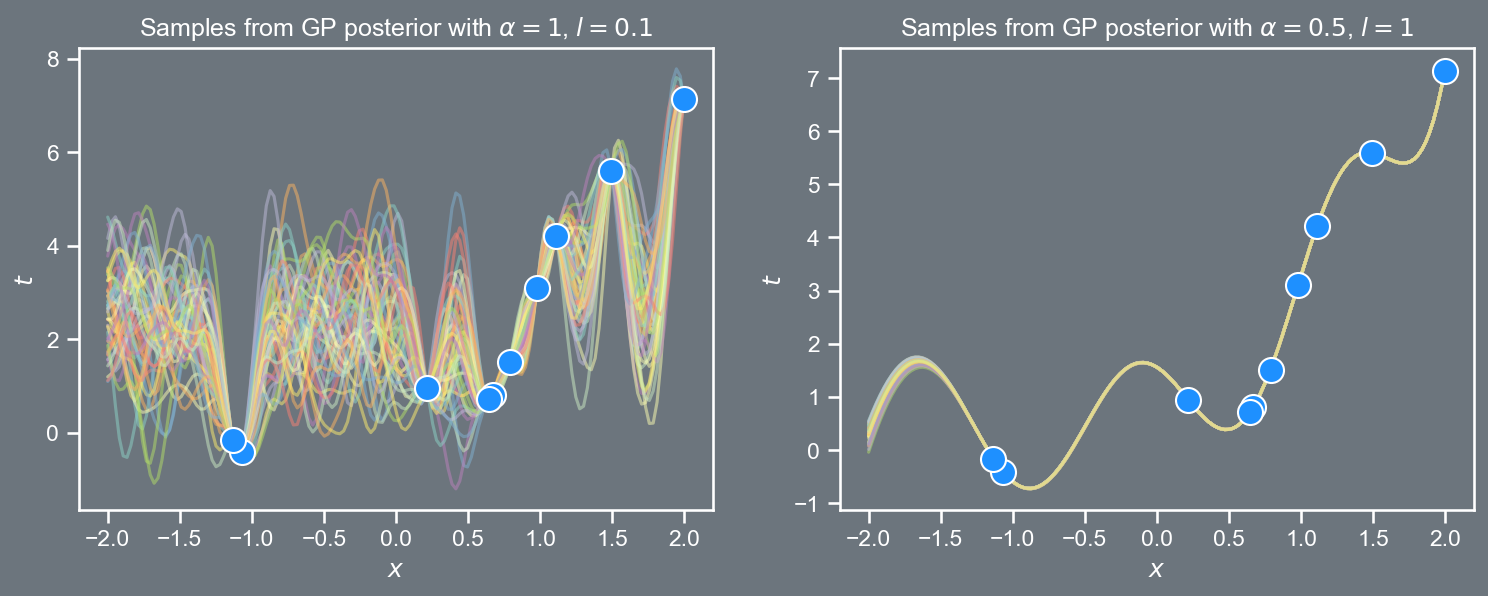
Visualizing GP posteriors
import pandas as pd
import numpy as np
import matplotlib
import matplotlib.pyplot as plt
from scipy.stats import multivariate_normal
from scipy.linalg import cholesky, solve_triangular
import seaborn as sns
sns.set(font_scale=1.0)
sns.set_style("white")
sns.set_style("ticks")
palette = sns.color_palette('deep')
plt.style.use('dark_background')


def kernel(xa, xb, amp, ll):
    Xa, Xb = get_tiled(xa, xb)
    return amp**2 * np.exp(-0.5 * 1./ll**2 * (Xa - Xb)**2 )

def get_tiled(xa, xb):
    m, n = len(xa), len(xb)
    xa, xb = xa.reshape(m,1) , xb.reshape(n,1)
    Xa = np.tile(xa, (1, n))
    Xb = np.tile(xb.T, (m, 1))
    return Xa, Xb

def get_posterior(amp, ll, x, x_data, y_data):
    u = y_data.shape[0]
    mu_y = np.mean(y_data)
    y = (y_data - mu_y).reshape(u,1)

    Kxx = kernel(x_data, x_data, amp, ll)
    Kxpx = kernel(x, x_data, amp, ll)
    Kxpxp = kernel(x, x, amp, ll)

    # Inverse
    jitter = np.eye(u) * 1e-8
    L = cholesky(Kxx + jitter)
    S1 = solve_triangular(L.T, y, lower=True)
    S2 = solve_triangular(L.T, Kxpx.T, lower=True).T

    mu = S2 @ S1  + mu_y
    cov = Kxpxp - S2 @ S2.T
    return mu, cov

x_data = np.random.rand(10)*4 - 2.
y_data = np.cos(5*x_data) + x_data**2 + 2*x_data
X = np.linspace(-2, 2, 150)
random_samples = 50

fig, ax = plt.subplots(2, figsize=(12,4))
fig.patch.set_facecolor('#6C757D')
ax[0].set_fc('#6C757D')
plt.subplot(121)
mu, cov = get_posterior(1, 0.1, X, x_data, y_data)
posterior = multivariate_normal(mu.flatten(), cov, allow_singular=True)
#mu = mu.flatten()
#std = np.sqrt(np.diag(cov)).flatten()
plt.plot(x_data, y_data, 'o', ms=12, color='dodgerblue', lw=1, markeredgecolor='w', zorder=3)
plt.plot(X, posterior.rvs(random_samples).T, alpha=0.5, zorder=2)
plt.title(r'Samples from GP posterior with $\alpha=1$, $l=0.1$')
plt.xlabel(r'$x$')
plt.ylabel(r'$t$')
#plt.ylabel(r'$\mathbf{w}_1$')
fig.patch.set_facecolor('#6C757D')

plt.subplot(122)
plt.rcParams['axes.facecolor']='#6C757D'
ax[1].set_facecolor('#6C757D')
mu2, cov2 = get_posterior(0.5, 1, X, x_data, y_data)
posterior2 = multivariate_normal(mu2.flatten(), cov2, allow_singular=True)
plt.plot(x_data, y_data, 'o', ms=12, color='dodgerblue', lw=1, markeredgecolor='w', zorder=3)
plt.plot(X, posterior2.rvs(random_samples).T, alpha=0.5, zorder=2)
plt.title(r'Samples from GP posterior with $\alpha=0.5$, $l=1$')
plt.xlabel(r'$x$')
plt.ylabel(r'$t$')
plt.savefig('posterior.png', dpi=150, bbox_inches='tight', facecolor="#6C757D")
plt.close()
An introduction to Gaussian processes
Kernel functions
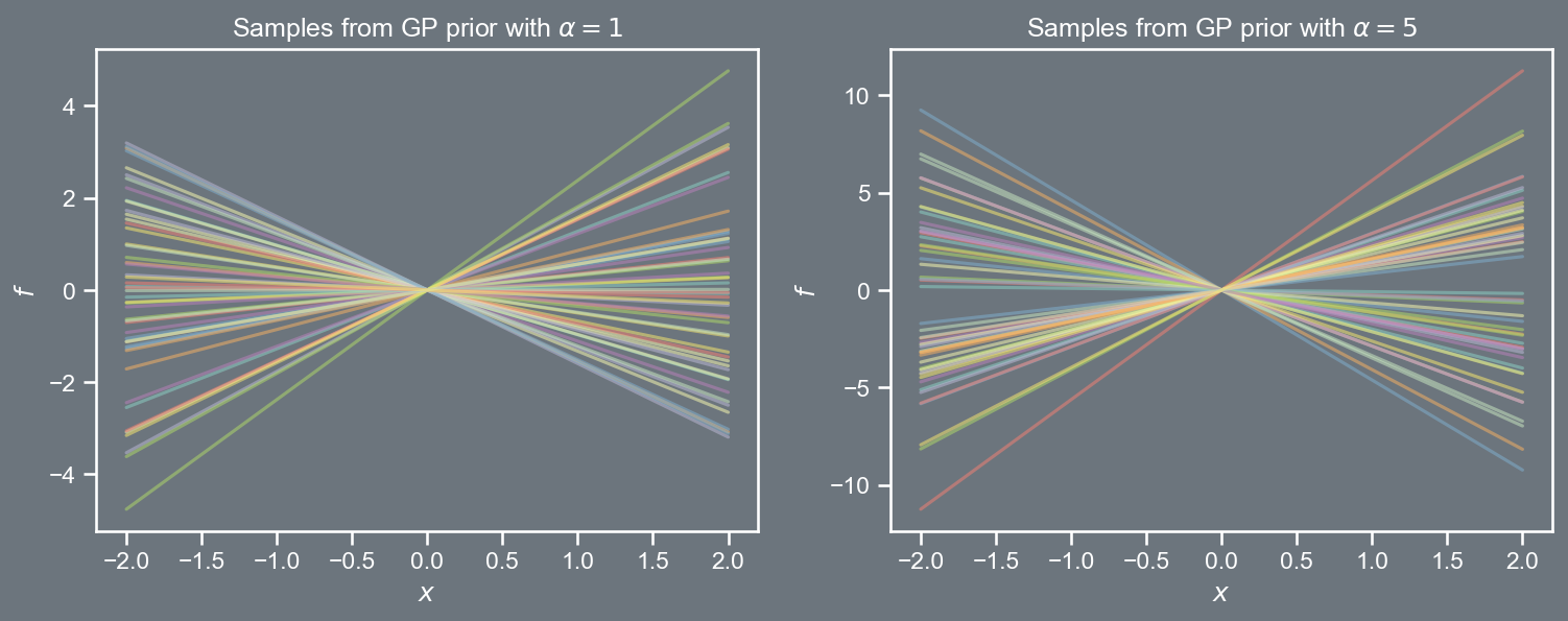
The RBF covariance function presented in the prior section is not the only candidate for a kernel function. Consider some of the other ones.
k \left( \boldsymbol{x}, \boldsymbol{x}' \right) = \alpha \; \boldsymbol{x}^{T} \boldsymbol{x}'
k \left( \boldsymbol{x}, \boldsymbol{x}' \right) = \alpha \; \left( 1 + \boldsymbol{x}^{T} \boldsymbol{x}' \right)^{\gamma}
k \left( \boldsymbol{x}, \boldsymbol{x}' \right) = \alpha^2 \; cos\left( \frac{2 \pi}{l^2} \left\Vert \boldsymbol{x} - \boldsymbol{x}' \right\Vert_{2}^{2} \right)