This assignment requires you to fit a Gaussian process model to the Mauna Loa data set. It is a univariate dataset that comprises the monthly average carbon dioxide concentration, measured in parts per million.
You will find the data at this site. You will have to download the monthly_in_situ_co2_mlo.csv file directly. Details about the data can be found in reference 1.
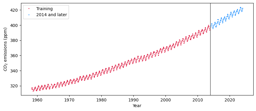
The plot below shows the data: year vs. CO2 (ppm). Some rows of the table have -99.99 values; these may be ignored. Note that as there are 12 measurements per year (1 for each month), utilizing just the year as the covariate is not appropriate, and that is why the “Date” or third column must be used.
Your training data must be limited to all years before 2014, i.e., you may only use CO2 concentrations in the years 1958 to 2013. It is entirely your decision whether you wish to use all this data, or select a subset.
A plot of all the data is shown below.
Code
import pandas as pdimport matplotlib.pyplot as pltimport numpy as npdf = pd.read_csv('data.csv')df2014 = df[df['Date']<2014]dfnew = df[df['Date']>=2014]fig = plt.figure(figsize=(10,4))plt.plot(df2014['Date'].values, df2014['CO2'].values, 'o', ms=1, color='crimson', label='Pre 2014 (training)')plt.plot(dfnew['Date'].values, dfnew['CO2'].values, 'o', ms=1, color='dodgerblue', label='2014 and later')plt.legend()plt.axvline(x=2014, color="grey")plt.xlabel('Year')plt.ylabel(r'$CO_2$ emissions (ppm)')plt.show()
Despite the fact that this is a univariate dataset, it is challenging as it requires multiple kernel functions. Ten minutes on your favorite search browser will give you some clues. Your grade will be determined via the following criterion.
Appropriate importing of the data and filtering of non-relevant rows. I will run your code on the “.csv” file as provided on the Scripps website. You cannot submit your amended version of the data.
Use of multiple kernel functions, justifying what exactly each kernel is doing.
A well-documented Jupyter notebook with equations for all the relevant formulas and code. If your code does not run, or produces an error upon running, you will loose a lot of marks.
One approach for hyperparameter inference (e.g., maximum likelihood, cross validation, Markov chain Monte Carlo, etc.). Please note that the signal noise need not be optimized over (but can be if you wish).
You will have to analytically calculate any gradients for hyperparameter inference. To clarify, code that does not use gradients, or code where the gradients are incorrect, will not receive full marks. To check your gradients you can always use finite differences.
You are restricted to the following libraries: numpy, seaborn, matplotlib, scipy, pandas. Thus, you will have to build a lot of the codebase yourself.
The last plot in your submission should have the same data as the plot above (both pre- and post-), along with predictive posterior mean and standard deviation contours.
Due date: 15th March 2024 | 21:00 on Canvas.
Grading rubric [marks in brackets]:
Data importing [5]
GP model architecture (i.e., kernels) [5]
Hyperparameter inference [10]
Clarity of documentation [5]
Reference
C. D. Keeling, S. C. Piper, R. B. Bacastow, M. Wahlen, T. P. Whorf, M. Heimann, and H. A. Meijer, Exchanges of atmospheric CO2 and 13CO2 with the terrestrial biosphere and oceans from 1978 to 2000. I. Global aspects, SIO Reference Series, No. 01-06, Scripps Institution of Oceanography, San Diego, 88 pages, 2001.