import numpy as np from scipy.stats import bernoulli, binom, exponimport matplotlib.pyplot as pltimport seaborn as snsfrom scipy.special import combsns.set(font_scale=1.0)sns.set_style("white")sns.set_style("ticks")palette = sns.color_palette('deep')
Problem 1
Find the probability density function of \(Y = h \left( X \right) = X^2\), for any \(y > 0\), where \(X\) is a continuous random variable with a known probability density function.
Solution
For \(y > 0\) we have
\[
F_Y \left( y \right) = p \left( Y \leq y \right) = p \left( X^2 \leq y \right) = p \left( - \sqrt{y} \leq X \leq \sqrt{y} \right)
\]
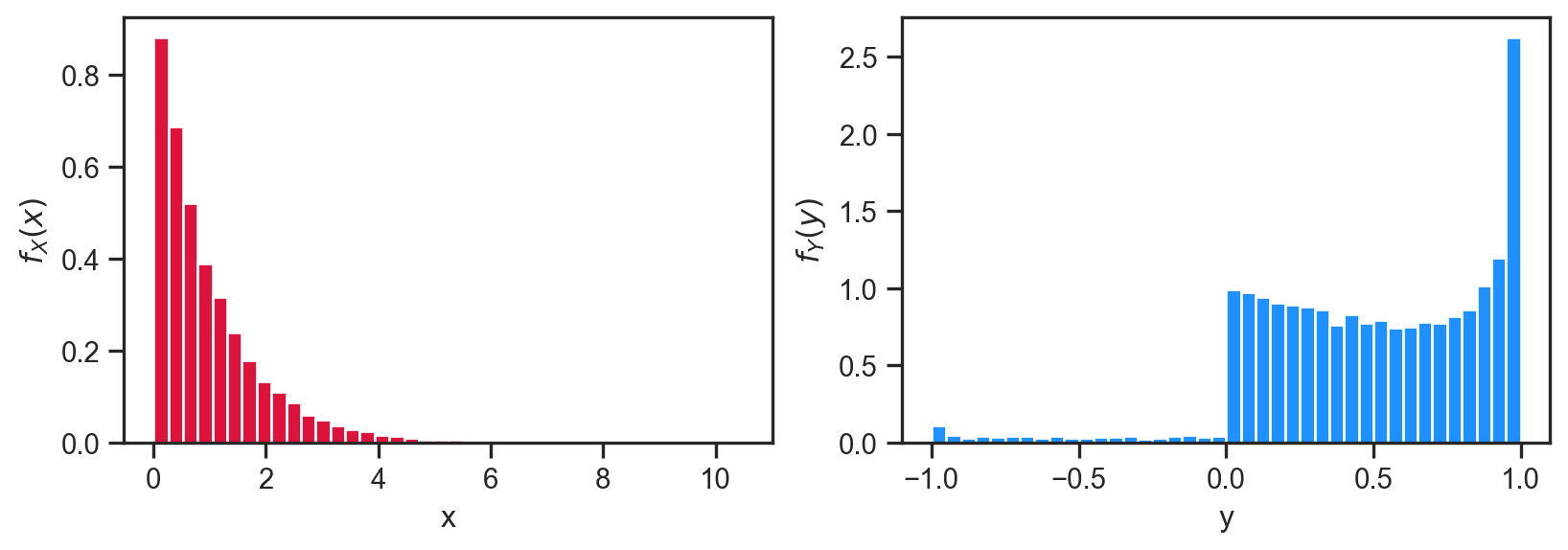
Following the bit of code above, let \(X\) be an exponential random variable with parameter \(\lambda\), i.e., \(f_{X} \left( x \right) = \lambda exp \left( -\lambda x \right)\) and \(F_{X} \left( x \right) = 1 - exp \left( -\lambda x \right)\). Let \(Y= sin\left( X \right)\). Determine \(F_Y\left( y \right)\) and \(f_{Y} \left( y \right)\).
Solution
From the event \(\left\{ Y \leq y \right\}\), we can conclude that for \(x = sin^{-1} \left( y \right)\) we have
\[
F_{Y} \left( y \right) = p \left( Y \leq y \right)
\]
\[
F_{Y} \left( y \right) = p \left( X \leq x \right) + \sum_{k=1}^{\infty} \left[ F_{X} \left( 2 k \pi + x \right) - F_{X} \left( \left(2k - 1 \right) \pi - x\right) \right]
\]
\[
F_{Y} \left( y \right) = p \left( X \leq x \right) + \sum_{k=1}^{\infty} \left[ 1 - exp\left( -\lambda x - 2 \lambda k \pi \right) - 1 + exp \left( \lambda x + \lambda \pi - 2 \lambda k \pi \right) \right]
\]
\[
= p \left( X \leq x \right) + \left[ exp\left( \lambda x \right) exp \left( \lambda \pi \right) - exp \left( - \lambda x \right) \right] \sum_{k=1}^{\infty} exp \left( - 2 \lambda k \pi \right)
\]
\[
= p \left( X \leq sin^{-1} \left( y \right) \right) + \left[ exp \left( \lambda sin^{-1} \left( y \right) + \lambda \pi \right) - exp \left( -\lambda sin^{-1} \left( y \right) \right) \right] \frac{exp \left( -2 \lambda \pi \right) }{1 - exp \left( -2 \lambda \pi \right)}
\]
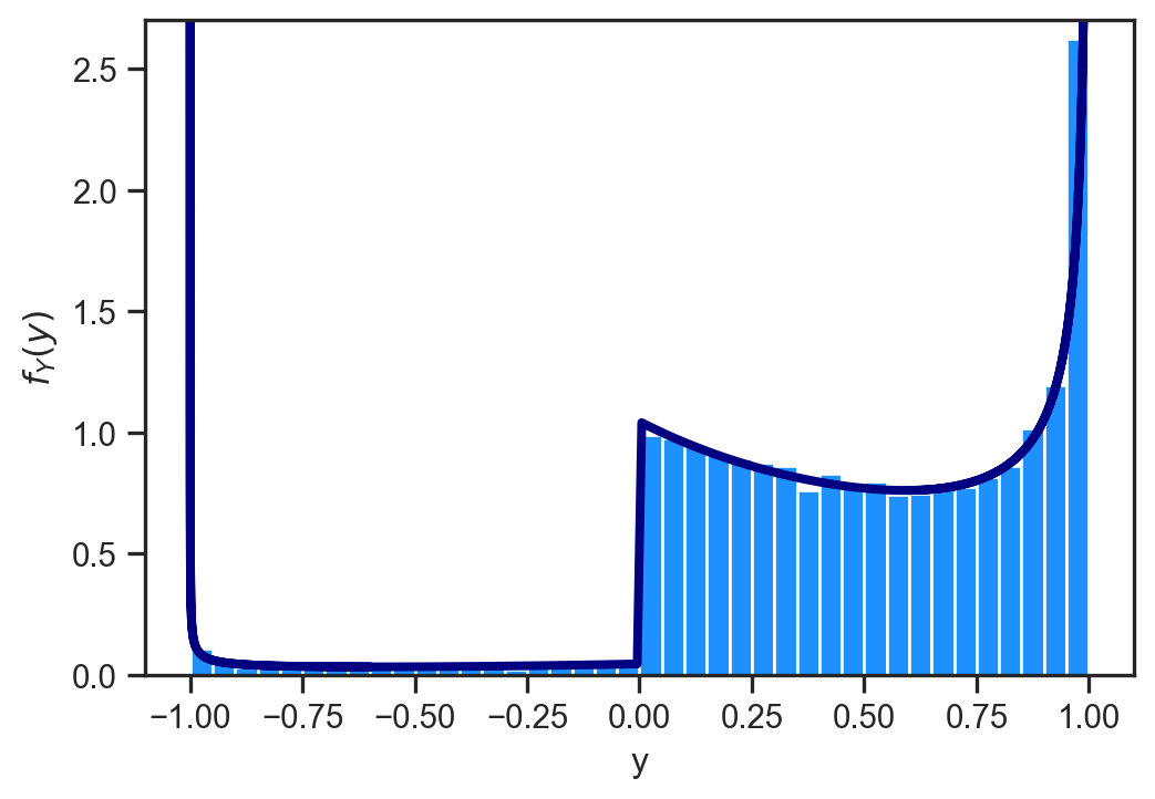
This expansion uses the sum of a geometric sequence formula. The first term above is zero for negative \(y \in [-1, 0)\) and
\[
p \left( X \leq sin^{-1} \left( y \right) \right) = F_{X} \left( sin^{-1} \left( y \right) \right) = 1 - exp(- \lambda sin^{-1}\left( y \right) )
\]
for non-negative \(y \in [0, 1]\). Since \(F_{X} \left(0\right) = 0\), the cumulative probability \(F_Y\left( y \right)\) will remain continuous at \(y=0\). However, its derivative is discontinuous and we will be unable to derive an expression for \(f_{Y} \left( 0 \right)\). Hence, for negative \(y \in [-1, 0)\) we have
Let \(X\) and \(Y\) be independent and uniform between \(0\) and \(1\). Compute \(X + Y\). To set the stage for the problem, consider the code and plot below.
Code
X = np.random.rand(9000)Y = np.random.rand(9000)S = X + Y fig = plt.figure(figsize=(6,3))plt.hist(X+Y,40, density=True, color='orangered')plt.ylabel(r'$f_{S}(s)$')plt.xlabel('s')plt.show()
It appears we have a triangular distribution. In what follows we shall aim to derive this analytically.
Solution
From the Lecture notes, we have:
\[
f_{S} \left( s \right) = \int_{0}^{1} f_{X} \left( x \right) f_{Y} \left( s - x \right) dx = \int_{0}^{1} f_{Y} \left( s - x \right) dx
\]
---title: "L4 examples"format: html: code-fold: truejupyter: python3fontsize: 1.2emlinestretch: 1.5toc: truenotebook-view: true---```{python}import numpy as np from scipy.stats import bernoulli, binom, exponimport matplotlib.pyplot as pltimport seaborn as snsfrom scipy.special import combsns.set(font_scale=1.0)sns.set_style("white")sns.set_style("ticks")palette = sns.color_palette('deep')```## Problem 1Find the probability density function of $Y = h \left( X \right) = X^2$, for any $y > 0$, where $X$ is a continuous random variable with a known probability density function. <details><summary>Solution</summary>For $y > 0$ we have$$F_Y \left( y \right) = p \left( Y \leq y \right) = p \left( X^2 \leq y \right) = p \left( - \sqrt{y} \leq X \leq \sqrt{y} \right)$$$$\Rightarrow F_Y \left( y \right) = F_{X} \left( \sqrt{y} \right) - F_{X} \left( - \sqrt{y} \right) $$Thus, by differentiating and applying the chain rule we have$$f_{Y} \left( y \right) = \frac{1}{2\sqrt{y}} f_{X} \left( \sqrt{y} \right) + \frac{1}{2 \sqrt{y}} f_{X} \left( - \sqrt{y} \right), \; \; \; \; y > 0 $$</details>## Problem 2Find the probability density function of $Y = exp \left( X^2 \right)$ if $X$ is a non-negative random variable. <details><summary>Solution</summary>Note that $F_Y \left( y \right) = 0$ for $y < 1$. For $y \geq 1$, we have$$F_{Y} \left( y \right) = p \left(exp \left(X^2 \right) \leq y \right) = p \left(X^2 \leq log \left( y \right) \right) $$$$\Rightarrow F_{Y} = p \left( X \leq \sqrt{log \left( y \right) } \right).$$By differentiating and using the chain rule, we obtain$$f_{Y} \left( y \right) = f_{X} \left( \sqrt{log \left( y \right) } \right) \frac{1}{2y \sqrt{log \left( y \right) } }, \; \; \; y > 1.$$</details>```{python}lam =1.X = expon.rvs(size=15000, scale=1/lam)Y = np.sin(X)fig = plt.figure(figsize=(10,3))plt.subplot(121)plt.hist(X,40, density=True, color='crimson')plt.ylabel(r'$f_{X}(x)$')plt.xlabel('x')plt.subplot(122)plt.hist(Y,40, density=True, color='dodgerblue')plt.ylabel(r'$f_{Y}(y)$')plt.xlabel('y')plt.show()```## Problem 3Following the bit of code above, let $X$ be an exponential random variable with parameter $\lambda$, i.e., $f_{X} \left( x \right) = \lambda exp \left( -\lambda x \right)$ and $F_{X} \left( x \right) = 1 - exp \left( -\lambda x \right)$. Let $Y= sin\left( X \right)$. Determine $F_Y\left( y \right)$ and $f_{Y} \left( y \right)$. <details><summary>Solution</summary>From the event $\left\{ Y \leq y \right\}$, we can conclude that for $x = sin^{-1} \left( y \right)$ we have$$F_{Y} \left( y \right) = p \left( Y \leq y \right)$$$$F_{Y} \left( y \right) = p \left( X \leq x \right) + \sum_{k=1}^{\infty} \left[ F_{X} \left( 2 k \pi + x \right) - F_{X} \left( \left(2k - 1 \right) \pi - x\right) \right]$$$$F_{Y} \left( y \right) = p \left( X \leq x \right) + \sum_{k=1}^{\infty} \left[ 1 - exp\left( -\lambda x - 2 \lambda k \pi \right) - 1 + exp \left( \lambda x + \lambda \pi - 2 \lambda k \pi \right) \right]$$$$= p \left( X \leq x \right) + \left[ exp\left( \lambda x \right) exp \left( \lambda \pi \right) - exp \left( - \lambda x \right) \right] \sum_{k=1}^{\infty} exp \left( - 2 \lambda k \pi \right) $$$$= p \left( X \leq sin^{-1} \left( y \right) \right) + \left[ exp \left( \lambda sin^{-1} \left( y \right) + \lambda \pi \right) - exp \left( -\lambda sin^{-1} \left( y \right) \right) \right] \frac{exp \left( -2 \lambda \pi \right) }{1 - exp \left( -2 \lambda \pi \right)}$$This expansion uses the *sum of a geometric sequence* formula. The first term above is zero for negative $y \in [-1, 0)$ and $$p \left( X \leq sin^{-1} \left( y \right) \right) = F_{X} \left( sin^{-1} \left( y \right) \right) = 1 - exp(- \lambda sin^{-1}\left( y \right) )$$for non-negative $y \in [0, 1]$. Since $F_{X} \left(0\right) = 0$, the cumulative probability $F_Y\left( y \right)$ will remain continuous at $y=0$. However, its derivative is discontinuous and we will be unable to derive an expression for $f_{Y} \left( 0 \right)$. Hence, for negative $y \in [-1, 0)$ we have$$f_{Y} \left( y \right) = \frac{d}{dx} F_{X} \left( x \right) \frac{dx}{dy} = \frac{\lambda}{\sqrt{1 - y^2}} \frac{exp \left( \lambda \left(sin^{-1} \left( y \right) + \pi \right) \right) + exp \left( -\lambda sin^{-1} \left( y \right) \right) }{exp \left( 2 \lambda \pi -1 \right) }.$$For positive $y \in (0, 1]$, we have$$f_{Y} \left( y \right) = \frac{d}{dx} F_{X} \left( x \right) \frac{dx}{dy} = \frac{\lambda}{\sqrt{1 - y^2}} \left[ \frac{exp \left( \lambda \left(sin^{-1} \left( y \right) + \pi \right) \right) + exp \left( -\lambda sin^{-1} \left( y \right) \right) }{exp \left( 2 \lambda \pi -1 \right) } + exp \left( -\lambda sin^{-1} \left( y \right) \right) \right].$$</details>```{python}x = np.linspace(-2.5, 2.5, 500)y = np.sin(x)def f_y(y): f_y = np.zeros((y.shape[0]))for i inrange(0, f_y.shape[0]):if y[i] >0: f_y[i] = lam/np.sqrt(1- y[i]**2) * (np.exp(-lam * np.arcsin(y[i])) \+ (np.exp(lam * np.arcsin(y[i]) + lam * np.pi) +\ np.exp(-lam * np.arcsin(y[i])))/(np.exp(2* lam * np.pi) -1))else: f_y[i] = lam/np.sqrt(1- y[i]**2) * ((np.exp(lam * np.arcsin(y[i]) + lam * np.pi) +\ np.exp(-lam * np.arcsin(y[i])))/(np.exp(2* lam * np.pi) -1))return f_yfig = plt.figure(figsize=(6,4))plt.plot(y, f_y(y), color='navy', lw=3)plt.hist(Y,40, density=True, color='dodgerblue')plt.ylabel(r'$f_{Y}(y)$')plt.xlabel('y')plt.ylim([0, 2.7])plt.show()```## Problem 4Let $X$ and $Y$ be independent and uniform between $0$ and $1$. Compute $X + Y$. To set the stage for the problem, consider the code and plot below. ```{python}X = np.random.rand(9000)Y = np.random.rand(9000)S = X + Y fig = plt.figure(figsize=(6,3))plt.hist(X+Y,40, density=True, color='orangered')plt.ylabel(r'$f_{S}(s)$')plt.xlabel('s')plt.show()```It appears we have a triangular distribution. In what follows we shall aim to derive this analytically.<details><summary>Solution</summary>From the Lecture notes, we have:$$f_{S} \left( s \right) = \int_{0}^{1} f_{X} \left( x \right) f_{Y} \left( s - x \right) dx = \int_{0}^{1} f_{Y} \left( s - x \right) dx$$$$\Rightarrow f_{S} \left( s \right) = \begin{cases}\begin{array}{c}\int_{0}^{s}1dx=s\\\int_{s-1}^{1}1dx=2-s\end{array} & \begin{array}{c}\textrm{for} \; \; s \in [0, 1]\\\textrm{for} \; \; s \in [1, 2]\end{array}\end{cases}$$</details>