This note concerns the Fourier dual of a kernel, i.e., one can think of a kernel has having an associated set of frequencies and amplitudes, much like studying the spectral density or power spectrum of a signal.
Code
import plotly.graph_objects as goimport plotly.figure_factory as ffimport plotly.express as pximport pandas as pdimport plotly.io as pioimport numpy as npfrom scipy.stats import multivariate_normalimport matplotlib.pyplot as pltpio.renderers.default ='iframe'from IPython.display import display, HTML
Bochner’s theorem
A stationary function \(k\left( \mathbf{x}, \mathbf{x}' \right)=k \left( \mathbf{x} - \mathbf{x}' \right) = k \left( \boldsymbol{\tau} \right)\) can be represented as the Fourier transform of a positive finite measure. The formal statement is given by
A complex-valued function \(k\) on \(\mathcal{X}\) is the covariance function of a weakly stationary mean square continuous complex-valued random process on \(\mathcal{X}\) if and only if it can be represented as
\[
k \left( \boldsymbol{\tau} \right) = \int_{\mathcal{X}} exp \left( 2 \pi i \boldsymbol{\omega} \cdot \boldsymbol{\tau} \right) d \mu \left( \boldsymbol{\omega} \right)
\]
where \(\mu\) is a positive finite measure, and \(\boldsymbol{\omega}\) are the frequencies. If \(\mu\) has a density \(S \left( \boldsymbol{\omega} \right)\), then \(S\) is the spectral density or power spectrum associated with the kernel \(k\).
Wiener-Khintchine theorem
A direct consequence of Bochner’s theoreom is the Wiener-Khintchine theorem. If the spectral density \(S \left( \boldsymbol{\omega} \right)\) exists, the spectral density and the covariance function are said to be Fourier duals. This leads to the following statement:
\[
k \left( \boldsymbol{\tau} \right) = \int S \left( \boldsymbol{\omega} \right) exp \left( 2 \pi i \boldsymbol{\omega} \cdot \boldsymbol{\tau} \right) d \boldsymbol{\omega}, \; \; \; \; S \left( \boldsymbol{\omega}\right) = \int k \left( \boldsymbol{\tau} \right) exp\left(- 2 \pi i \boldsymbol{\omega} \cdot \boldsymbol{\tau} \right) d \boldsymbol{\tau}
\]
As noted in RW, \(S \left( \boldsymbol{\omega} \right)\) is essentially the amount of power assigned to the eigenfunction \(exp \left( 2 \pi i \boldsymbol{\omega} \cdot \mathbf{\tau} \right)\) with frequency \(\boldsymbol{\omega}\). The amplitude as a function of frequency \(S\left( \boldsymbol{\omega} \right)\) must decay sufficiently fast so that the terms above are integrable.
There are some important points to note:
If we have a stationary kernel, we can resolve what frequencies underscore the model by working out its Fourier transform.
On the other hand, if we have a certain spectral density of interest, then its inverse Fourier transform is a kernel.
To analytically work this out, it may be useful to go through an example (courtsey of Markus Heinonen). The derivation below will require three pieces: - We shall assume a symmetric frequency distribution, i.e., \(S\left( \boldsymbol{\omega} \right) = S \left( -\boldsymbol{\omega} \right)\). - From Euler’s formula we have \(cos\left(x\right) \pm i sin\left(x \right) = exp \left(\pm ix \right)\) - The negative sine identity, i.e., \(sin \left( -x \right) = - sin \left( x \right)\)
Starting with the expression above, we begin wtih
\[
\begin{aligned}
k \left( \boldsymbol{\tau} \right) & = \int_{-\infty}^{\infty} S \left( \boldsymbol{\omega} \right) exp \left( 2 \pi i \boldsymbol{\omega} \cdot \boldsymbol{\tau} \right) d \boldsymbol{\omega} \\
& = \int_{-\infty}^{\infty} S \left(\boldsymbol{\omega} \right) cos \left( 2 \pi\boldsymbol{\tau} \cdot \boldsymbol{\omega} \right) d \boldsymbol{\omega} + \int_{-\infty}^{\infty} iS \left(\boldsymbol{\omega} \right) sin \left( 2 \pi \boldsymbol{\tau} \cdot \boldsymbol{\omega} \right) d \boldsymbol{\omega} \\
& = \mathbb{E}\left[ S \left(\omega \right) \right] cos \left( 2 \pi \boldsymbol{\tau} \cdot \boldsymbol{\omega} \right) + \int_{-\infty}^{0} iS \left(\boldsymbol{\omega} \right) sin \left( 2 \pi \boldsymbol{\tau} \cdot \boldsymbol{\omega} \right) d \boldsymbol{\omega} + \int_{0}^{\infty} iS \left(\boldsymbol{\omega} \right) sin \left( 2 \pi \boldsymbol{\tau} \cdot \boldsymbol{\omega} \right) d \boldsymbol{\omega} \\
& = \mathbb{E}\left[ S \left(\omega \right) \right] cos \left( 2 \pi \boldsymbol{\tau} \cdot \boldsymbol{\omega} \right) + \int_{0}^{\infty} iS \left(-\boldsymbol{\omega} \right) sin \left( -2 \pi \boldsymbol{\tau} \cdot \boldsymbol{\omega} \right) d \boldsymbol{\omega} + \int_{0}^{\infty} iS \left(\boldsymbol{\omega} \right) sin \left( 2 \pi \boldsymbol{\tau} \cdot \boldsymbol{\omega} \right) d \boldsymbol{\omega} \\
& = \mathbb{E}\left[ S \left(\omega \right) \right] cos \left( 2 \pi \boldsymbol{\tau} \cdot \boldsymbol{\omega} \right) + \int_{0}^{\infty} -iS \left(\boldsymbol{\omega} \right) sin \left( 2 \pi \boldsymbol{\tau} \cdot \boldsymbol{\omega} \right) d \boldsymbol{\omega} + \int_{0}^{\infty} iS \left(\boldsymbol{\omega} \right) sin \left( 2 \pi \boldsymbol{\tau} \cdot \boldsymbol{\omega} \right) d \boldsymbol{\omega} \\
\end{aligned}
\]
This leads to
\[
\begin{aligned}
k \left( \boldsymbol{\tau} \right) & = \mathbb{E}\left[ S \left(\omega \right) \right] cos \left( 2 \pi \boldsymbol{\tau} \cdot \boldsymbol{\omega} \right)
\end{aligned}
\]
This demonstrates that all real-valued stationary kernels are \(S\left( \boldsymbol{\omega} \right)\)-weighted combinations of cosine terms.
Kernel harmonic representation
Our new general stationary kernel definition is thus:
\[
k \left( \boldsymbol{\tau} \right) = \mathbb{E}\left[ S \left(\omega \right) \right] cos \left( 2 \pi \boldsymbol{\tau} \cdot \boldsymbol{\omega} \right)
\]
where the frequencies \(\boldsymbol{\omega}\) are an inverse of the period \(1/\boldsymbol{\omega}\). Bracewell provides the following expressions for the Wiener-Khintchine result, by integrating out the angular variables (see page 83 of RW):
\[
\begin{aligned}
k \left( \boldsymbol{\tau} \right) & = \frac{2 \pi}{\boldsymbol{\tau}^{-1/2}} \int_{0}^{\infty} S \left( \boldsymbol{\omega} \right) J_{-1/2} \left(2 \pi \boldsymbol{\tau} \cdot \boldsymbol{\omega} \right) \boldsymbol{\omega}^{1/2} d \boldsymbol{\omega} \\
S \left( \boldsymbol{\omega} \right) & = \frac{2 \pi}{\boldsymbol{\omega}^{-1/2}} \int_{0}^{\infty} k \left( \boldsymbol{\tau} \right) J_{-1/2} \left(2 \pi \boldsymbol{\tau} \cdot \boldsymbol{\omega} \right) \boldsymbol{\tau}^{1/2} d \boldsymbol{\tau}
\end{aligned}
\]
Note that in RW, the authors use \(D\) to denote the dimensionality, which we have assumed to be 1. The function \(J_{-1/2}\) is the Bessel function of order \(-1/2\). While the expressions above may seem unwiedly, we can work out what these are using a bit of Sympy. Consider the case of a squared exponential kernel of the form
\[
k \left(\boldsymbol{\tau} \right) = exp \left(- \frac{\boldsymbol{\tau}^2}{2l^2} \right).
\]
Notice that the more terms we incorporate, the closer we converge to the true kernel.
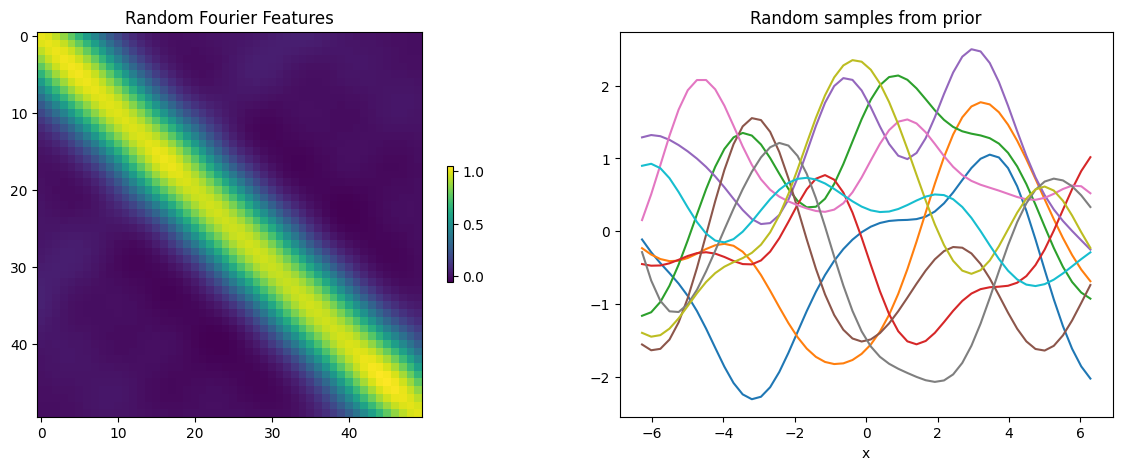
Random Fourier Features
Rather than negotiate a kernel approximation with a great many number of terms, it will be more instructive to resort to a few terms. Such is the idea behind Random Fourier Features, where one selects a kernel comprised of random frequencies. For more details, please see the paper by Rahimi and Recht.
Code
R =500# random featuresD =50# number of data pts.x = np.linspace(-2*np.pi, 2*np.pi, D).reshape(D,1) # gridX = np.tile(x, [1, D]) - np.tile(x.T, [D, 1])W = np.random.normal(loc=0, scale=0.1, size=(R, D))b = np.random.uniform(0, 2*np.pi, size=R)B = np.repeat(b[:, np.newaxis], D, axis=1)norm =1./ np.sqrt(R)Z = norm * np.sqrt(2) * np.cos(W @ X.T + B)ZZ = Z.T @ Z