Incompressible fluid mechanics

Problem 1

A mixing tank has two inlets and one outlet, all of the same area, \(0.01 \; m^2\). Liquids of density \(\require{color}{\color[rgb]{0.918231,0.469102,0.038229}\rho_1 } = {\color[rgb]{0.918231,0.469102,0.038229}800 \; kg/m^3}\) and \(\require{color}{\color[rgb]{0.918231,0.469102,0.038229}\rho_2 } = {\color[rgb]{0.918231,0.469102,0.038229}900 \; kg/m^3}\) flow into the tank through separate inlets. They have uniform inlet velocities of \(\require{color}{\color[rgb]{0.059472,0.501943,0.998465}3.1 \; m/s}\) and \(\require{color}{\color[rgb]{0.059472,0.501943,0.998465}1.9 \; m/s}\) respectively. Mixing is assumed to be complete, and the conditions at the tank outlet are uniform. Assuming steady state conditions, find

• the mass flows into and out of the tank

• the mean density and velocity of the mixture flowing out of the tank

Note that the mean velocity can be calculated based on the assumption of incompressible flow.

Solution

Consider the schematic shown below.

\[ \large \require{color}\dot{m}_{1} = {\color[rgb]{0.918231,0.469102,0.038229}\rho_1 } A {\color[rgb]{0.059472,0.501943,0.998465}v_1}, \; \; \; \require{color}\dot{m}_{2} = {\color[rgb]{0.918231,0.469102,0.038229}\rho_2 } A {\color[rgb]{0.059472,0.501943,0.998465}v_2} \]

As conservation of mass must hold within the control volume, we have

\[ \large \require{color}\dot{m}_{1} + \dot{m}_{2} = \dot{m}_{3} \]

Note that since both liquids flowing into the tank are incompressible, we can use volumetric flow rates, i.e.,

\[ \large \require{color}A {\color[rgb]{0.059472,0.501943,0.998465}v_1} + A {\color[rgb]{0.059472,0.501943,0.998465}v_2} = A {\color[rgb]{0.059472,0.501943,0.998465}v_3} \]

Noting that the areas are the same,

\[ \large \require{color}{\color[rgb]{0.059472,0.501943,0.998465}v_1} + {\color[rgb]{0.059472,0.501943,0.998465}v_2} = {\color[rgb]{0.059472,0.501943,0.998465}v_3} \]

Assigning values to the equations above, yields:

Code

v_1 = 3.1
v_2 = 1.9
rho_1 = 800
rho_2 = 900
A = 0.01

# From the equations above, we have the massflows in and out of the tank to be:
m_1 = rho_1 * v_1 * A
m_2 = rho_2 * v_2 * A
m_3 = m_1 + m_2

print('The massflows are: m_1 '+str(m_1)+' kg/s, m_2 '+str(m_2)+' kg/s, and m_3 '+str(m_3)+' kg/s')
v_3 = v_1 + v_2
rho_3 = m_3 / (v_3 * A)

print('The mass density of the outflow is '+str(rho_3)+' kg/m^3, with a velocity of '+str(v_3)+' m/s')

The massflows are: m_1 24.8 kg/s, m_2 17.1 kg/s, and m_3 41.900000000000006 kg/s
The mass density of the outflow is 838.0000000000001 kg/m^3, with a velocity of 5.0 m/s

Problem 2

A cylindrical tank with base area \(A\) and maximum height \(H\) receives a steady flow rate \(\dot{m}_1\) from a tank, and drains a mass flow rate \(\dot{m}_2\). The inlet pipe has a radius \(R\) and uniform velocity \(\require{color}{\color[rgb]{0.059472,0.501943,0.998465}V_0 \; m/s}\). The outlet pipe also has the same radius \(R\) and a velocity profile

\[ \large \require{color}{\color[rgb]{0.059472,0.501943,0.998465}v}(r)={\color[rgb]{0.059472,0.501943,0.998465}V_0 } \left( 1- \left( \frac{r}{R} \right)^2 \right) \]

At time \(t = 0\), the volume of liquid in the tank is at level \(h_o\) from the base. The density of the fluid is constant and equal to \(\require{color}{\color[rgb]{0.918231,0.469102,0.038229}\rho}\). In each case, determine the expression as a function of \(R, {\color[rgb]{0.059472,0.501943,0.998465}V_0 }, A, H, ho,\) and \(\require{color}{\color[rgb]{0.918231,0.469102,0.038229}\rho}\).

• Determine the mass flow rates through the inlet and outlet.

• Determine the rate of mass accumulation in the tank.

Solution

To begin, consider the schematic above. Recognize that the massflow rate going into the tank is given by

\[ \large \require{color}\dot{m}_1 = {\color[rgb]{0.918231,0.469102,0.038229}\rho}A_1 {\color[rgb]{0.059472,0.501943,0.998465}v_1} = {\color[rgb]{0.918231,0.469102,0.038229}\rho} \pi R^2 {\color[rgb]{0.059472,0.501943,0.998465}V_0 }. \]

The massflow rate leaving the tank is given by:

\[ \large \require{color}\dot{m}_2 = \int {\color[rgb]{0.918231,0.469102,0.038229}\rho} {\color[rgb]{0.059472,0.501943,0.998465}v} dA = \int_{0}^{R} {\color[rgb]{0.918231,0.469102,0.038229}\rho} {\color[rgb]{0.059472,0.501943,0.998465}v}(r) 2 \pi r dr \]

\[ \large \require{color}\dot{m}_2 = \int_{0}^{R} {\color[rgb]{0.918231,0.469102,0.038229}\rho} {\color[rgb]{0.059472,0.501943,0.998465}V_0 } \left( 1- \left( \frac{r}{R} \right)^2 \right) 2 \pi r dr \]

\[ \large \require{color}\dot{m}_2 = {\color[rgb]{0.918231,0.469102,0.038229}\rho} {\color[rgb]{0.059472,0.501943,0.998465}V_0 } 2 \pi \left[ \frac{r^2}{2} - \frac{r^4}{4R^2} \right]^{R}_{0} = {\color[rgb]{0.918231,0.469102,0.038229}\rho} {\color[rgb]{0.059472,0.501943,0.998465}V_0 } \pi \frac{R^2}{2} \]

The mass accumulation in the tank is given by

\[ \large \require{color}\frac{dm}{dt} = \dot{m}_1 - \dot{m}_2 = {\color[rgb]{0.918231,0.469102,0.038229}\rho} \pi R^2 {\color[rgb]{0.059472,0.501943,0.998465}V_0 } - {\color[rgb]{0.918231,0.469102,0.038229}\rho} {\color[rgb]{0.059472,0.501943,0.998465}V_0 } \pi \frac{R^2}{2} = {\color[rgb]{0.918231,0.469102,0.038229}\rho} {\color[rgb]{0.059472,0.501943,0.998465}V_0 } \pi \frac{R^2}{2} \]

Problem 3

A submerged submarine is towed horizontally at a steady speed \(\require{color}{\color[rgb]{0.059472,0.501943,0.998465}U}\) in deep, still water. Far behind at a fixed distance from the submarine an axially-symmetrical wake is formed in which the water velocity may be assumed to vary from \(\require{color}{\color[rgb]{0.059472,0.501943,0.998465}U}\) on the axis to zero at radius R (see schematic) as follows:

\[ \large \require{color}{\color[rgb]{0.059472,0.501943,0.998465}u}(r)={\color[rgb]{0.059472,0.501943,0.998465}U } \left( 1- \left( \frac{r}{R} \right)^2 \right) \]

The variation of the water pressure with depth may be assumed to be unaffected by the presence of the submarine. The density of the water is \(\require{color}{\color[rgb]{0.918231,0.469102,0.038229}\rho}\).

• To use the continuity and steady flow momentum equations we employ a moving control volume, in which the submarine appears stationary. Why do we need to do this? What is the velocity distribution in the wake relative to the moving control volume?

• Show that the drag on the submarine is given by:

\[ \large \require{color}{\color[rgb]{0.986252,0.007236,0.027423}F_{d}} = \frac{1}{6} \pi {\color[rgb]{0.918231,0.469102,0.038229}\rho }{\color[rgb]{0.059472,0.501943,0.998465}U}^2 R^2 \]

Hint: Before applying momentum equation, make sure all mass flows are accounted for in the control volume used. There are two obvious control volumes to take, which should give the same answer.

Submarine	Schematc

Solution

A moving control volume is required to make this a steady flow problem. Consider a control volume moving with speed \(\require{color}{\color[rgb]{0.059472,0.501943,0.998465}u}(r)={\color[rgb]{0.059472,0.501943,0.998465}U}\).

Here the velocity is given by

\[ \large \require{color}{\color[rgb]{0.059472,0.501943,0.998465}u}(r)={\color[rgb]{0.059472,0.501943,0.998465}U } \left( \frac{r}{R} \right)^2 \]

where \(r\) goes from \(0\) to \(R\). We can define a cylindrical volume that is created by the submarine, where the velocity profile essentially mirrors that of the expression above.

Now as we are only interested in the momentum along the horizontal direction, we can neglect the hydrostatic pressure contributions as they are the same at both ends.

The first task is to apply continuity to quantify the massflow out of the side of the control volume. This is because the inflow at the front is not equal to the outflow at the rear. The fluid that leaves the sides does have momentum along the horizontal direction. At the inlet, we have

\[ \large \require{color}\dot{m}_{in} = {\color[rgb]{0.918231,0.469102,0.038229}\rho } \pi R^2 {\color[rgb]{0.059472,0.501943,0.998465}U } \]

and at the outflow at the rear:

\[ \large \require{color}\dot{m}_{out} = \int_{0}^{R} {\color[rgb]{0.918231,0.469102,0.038229}\rho } {\color[rgb]{0.059472,0.501943,0.998465}U } \left(\frac{r}{R} \right)^2 2 \pi r dr = \int_{0}^{R} {\color[rgb]{0.918231,0.469102,0.038229}\rho } {\color[rgb]{0.059472,0.501943,0.998465}U } 2 \pi \frac{r^3}{R^2}dr = \frac{1}{2} {\color[rgb]{0.918231,0.469102,0.038229}\rho } \pi R^2 {\color[rgb]{0.059472,0.501943,0.998465}U } \]

From conservation of mass, we know that the massflow that exits at the sides must be

\[ \large \require{color}\dot{m}_{sides} = \dot{m}_{out} - \dot{m}_{in} = \frac{1}{2} {\color[rgb]{0.918231,0.469102,0.038229}\rho } \pi R^2 {\color[rgb]{0.059472,0.501943,0.998465}U }. \]

To work out the drag, we setup the steady flow momentum equation along the horizontal direction, recognizing that the drag force is pointing along the positive horizontal direction (given that in our control volume the velocity is pointing along the negative horizontal direction).

\[ \large \require{color}F_{{\color[rgb]{0.986252,0.007236,0.027423}d}} = \sum \dot{m}_{out} {\color[rgb]{0.059472,0.501943,0.998465}v_{out}} - \sum \dot{m}_{in} {\color[rgb]{0.059472,0.501943,0.998465}v_{in}} \]

\[ \large \require{color}F_{{\color[rgb]{0.986252,0.007236,0.027423}d}} = \underbrace{-\int {\color[rgb]{0.918231,0.469102,0.038229}\rho} {\color[rgb]{0.059472,0.501943,0.998465}u}^2 dA }_{\textsf{outflow at back less than zero (neg. vel)}} + \underbrace{\dot{m}_{side}\left(-{\color[rgb]{0.059472,0.501943,0.998465}U} \right)}_{\textsf{outflow on sides}} - \underbrace{\dot{m}_{in} \left(-{\color[rgb]{0.059472,0.501943,0.998465}U} \right)}_{\textsf{inflow at front}} \]

\[ \large \require{color}F_{{\color[rgb]{0.986252,0.007236,0.027423}d}} = -\int_{0}^{R} {\color[rgb]{0.918231,0.469102,0.038229}\rho } \left( {\color[rgb]{0.059472,0.501943,0.998465}U } \left( \frac{r}{R} \right)^2 \right)^2 2 \pi r dr + \frac{1}{2} {\color[rgb]{0.918231,0.469102,0.038229}\rho } \pi R^2 {\color[rgb]{0.059472,0.501943,0.998465}U} \left(-{\color[rgb]{0.059472,0.501943,0.998465}U}\right) + {\color[rgb]{0.918231,0.469102,0.038229}\rho } \pi R^2 {\color[rgb]{0.059472,0.501943,0.998465}U}^2 \]

\[ \large \require{color}F_{{\color[rgb]{0.986252,0.007236,0.027423}d}} = \frac{1}{2} {\color[rgb]{0.918231,0.469102,0.038229}\rho } \pi R^2 {\color[rgb]{0.059472,0.501943,0.998465}U}^2 - \frac{2 \pi {\color[rgb]{0.918231,0.469102,0.038229}\rho {\color[rgb]{0.059472,0.501943,0.998465}U}^2} }{R^4} \left[ \frac{R^6}{6} \right] \]

\[ \large \require{color}F_{{\color[rgb]{0.986252,0.007236,0.027423}d}} = \frac{1}{6}\pi {\color[rgb]{0.918231,0.469102,0.038229}\rho {\color[rgb]{0.059472,0.501943,0.998465}U}}^2 R^2 \]

Problem 4

Two parallel streams of an incompressible fluid flowing in horizontal rectangular ducts of height \(h\) and depth \(d\) come together at the location \(AA'\) as shown in the figure. They have the same static pressure \(\require{color}{\color[rgb]{0.315209,0.728565,0.037706}p_{A}}\) and speeds \(V\) and \(3V\) respectively. The two streams mix over a short distance due to the turbulence generated by the unstable shear layer between them.

Assuming the viscous shear stress on the solid surfaces can be neglected, calculate the velocity and static pressure at location \(BB'\), where the mixing is complete.

Solution

To work out the velocity, we use conservation of mass, i.e.,

\[ \large \require{color} \require{color}{\color[rgb]{0.918231,0.469102,0.038229}\rho} {\color[rgb]{0.059472,0.501943,0.998465}V } dh + \require{color}{\color[rgb]{0.918231,0.469102,0.038229}\rho}{\color[rgb]{0.059472,0.501943,0.998465}3V } dh = \require{color}{\color[rgb]{0.918231,0.469102,0.038229}\rho} {\color[rgb]{0.059472,0.501943,0.998465}V'} d 2h \]

\[ \large \require{color} \Rightarrow {\color[rgb]{0.059472,0.501943,0.998465}V'} = {\color[rgb]{0.059472,0.501943,0.998465}2V} \]

where \(\require{color}{\color[rgb]{0.059472,0.501943,0.998465}V'}\) is the exit velocity.

To work out the static pressure, we use the conservation of momentum, i.e., the force on the control volume is the net flow of momentum out.

\[ \large \require{color}{\color[rgb]{0.315209,0.728565,0.037706}p_{A}} 2hd - {\color[rgb]{0.315209,0.728565,0.037706}p_{B}}2hd = {\color[rgb]{0.918231,0.469102,0.038229}\rho}{\color[rgb]{0.059472,0.501943,0.998465}V'} 2hd{\color[rgb]{0.059472,0.501943,0.998465}V'} - {\color[rgb]{0.918231,0.469102,0.038229}\rho} {\color[rgb]{0.059472,0.501943,0.998465}V} hd{\color[rgb]{0.059472,0.501943,0.998465}V} - {\color[rgb]{0.918231,0.469102,0.038229}\rho} 3{\color[rgb]{0.059472,0.501943,0.998465}V} hd3{\color[rgb]{0.059472,0.501943,0.998465}V} \]

\[ \large \require{color} {\color[rgb]{0.315209,0.728565,0.037706}p_{A}} - {\color[rgb]{0.315209,0.728565,0.037706}p_{B}} = \frac{{\color[rgb]{0.918231,0.469102,0.038229}\rho} h d}{2 h d}\left[ 2 \left(2 {\color[rgb]{0.059472,0.501943,0.998465}V}\right)^2 - {\color[rgb]{0.059472,0.501943,0.998465}V}^2 - 9{\color[rgb]{0.059472,0.501943,0.998465}V}^2\right] = - \frac{2 {\color[rgb]{0.918231,0.469102,0.038229}\rho} h d{\color[rgb]{0.059472,0.501943,0.998465}V}^2}{2hd} \]

\[ \large \require{color} {\color[rgb]{0.315209,0.728565,0.037706}p_{B}} = {\color[rgb]{0.315209,0.728565,0.037706}p_{A}} + {\color[rgb]{0.918231,0.469102,0.038229}\rho} {\color[rgb]{0.059472,0.501943,0.998465}V}^2 \]

{p}

Problem 5

Consider a nozzle as shown in the diagram in below. The nozzle converges gradually, and we assume that the flow in it is:

• approximately uniform over any particular horizontal station \(x\);
• it is incompressible;
• it is inviscid, and
• any gravitational effects are negligible.

The volumetric flow rate in the nozzle is given as \(Q\) and the ambient pressure is \(p_a\).

• Derive an expression for the gauge pressure at a horizontal station where the area is \(A\left(x\right)\).

• Show by integrating the \(x-\)component of the pressure force on the nozzle’s interior walls, that the net \(x-\)component of force on the nozzle due to the flow is independent of the specific nozzle contour and is given by

\[ \large F = \rho Q^2 \frac{\left(A_{inlet} - A_2\right)^2}{2A_{inlet} A^2_2} \]

where \(A_2\) is the area at the exit and \(A_{inlet}\) is the area at the inlet.

Solution

While it is natural to apply Bernoulli’s principle to such a problem, let us clarify why. Consider all the assumptions that underscore Bernoulli, i.e., the flow must be

• inviscid;
• along a streamline (satisfied by the fact that we are told the flow is approximately uniform);
• steady;
• constant density;
• no work / energy input or loss (e.g., there is no friction).

This enables us to write:

\[ \large \require{color} \underbrace{p\left(x\right) + \frac{1}{2}{\color[rgb]{0.918231,0.469102,0.038229}\rho} {\color[rgb]{0.059472,0.501943,0.998465}v}^2\left(x\right)}_{\textsf{station 1}} = \underbrace{{\color[rgb]{0.315209,0.728565,0.037706}p}_{a} + \frac{1}{2}{\color[rgb]{0.918231,0.469102,0.038229}\rho} {\color[rgb]{0.059472,0.501943,0.998465}v'}_{2}^2}_{\textsf{station 2}} \]

\[ \large \require{color} {\color[rgb]{0.315209,0.728565,0.037706}p}\left(x\right) - {\color[rgb]{0.315209,0.728565,0.037706}p}_a = \frac{1}{2}{\color[rgb]{0.918231,0.469102,0.038229}\rho} \left( {\color[rgb]{0.059472,0.501943,0.998465}v}_2^2 - {\color[rgb]{0.059472,0.501943,0.998465}v}^2\left(x\right)\right) \]

The gauge pressure \({\color[rgb]{0.315209,0.728565,0.037706}p}_{g}\) is defined as the atmospheric pressure subtracted from a measured pressure, i.e.,

\[ \large \require{color} {\color[rgb]{0.315209,0.728565,0.037706}p}_{g} = {\color[rgb]{0.315209,0.728565,0.037706}p}\left( x \right) - {\color[rgb]{0.315209,0.728565,0.037706}p}_a \]

\[ \large \require{color} = \frac{1}{2}\rho \left({\color[rgb]{0.059472,0.501943,0.998465}v}_2^2 - {\color[rgb]{0.059472,0.501943,0.998465}v}^2\left(x\right) \right) \]

Recognising that the velocity may be written as

\[ \large \require{color} {\color[rgb]{0.059472,0.501943,0.998465}v}\left(x\right) = \frac{Q}{A\left(x\right)} \]

we have

\[ \large \require{color} {\color[rgb]{0.315209,0.728565,0.037706}p}_g = \frac{1}{2}{\color[rgb]{0.918231,0.469102,0.038229}\rho} \left({\color[rgb]{0.059472,0.501943,0.998465}v}_2^2 - \frac{Q^2}{A^2\left(x\right)} \right) = \frac{1}{2}{\color[rgb]{0.918231,0.469102,0.038229}\rho} Q^2 \left(\frac{1}{A_2^2} - \frac{1}{A^2\left(x\right)} \right) . \]

The question asks us to integrate the \(x-\)component of the pressure force, i.e.,

\[ \large \require{color} \int_{inlet}^{2^{\ast}} {\color[rgb]{0.315209,0.728565,0.037706}p}_{g}\left(x\right) dA = F_{pressure,x} \]

We still need to work out the relevant length along the vertical direction; see the Figure below.

\[ \large \require{color} F_{pressure,x} = \int_{A_{inlet}}^{A_2} {\color[rgb]{0.315209,0.728565,0.037706}p}_{g} \; d\left[A_{inlet} - A \right] \]

\[ \large \require{color} = -\int_{A_{inlet}}^{A_2} {\color[rgb]{0.315209,0.728565,0.037706}p}_{g} \; dA \]

\[ \large \require{color} = -\frac{{\color[rgb]{0.918231,0.469102,0.038229}\rho} Q^2}{2} \int_{A_{inlet}}^{A_2} \left(\frac{1}{A_2^2} - \frac{1}{A^2\left(x\right)} \right)dA \]

\[ \large \require{color} =-\frac{{\color[rgb]{0.918231,0.469102,0.038229}\rho} Q^2}{2} \left\{ \left[ \frac{A}{A_2^2}\right]_{A_{inlet}}^{A_2} - \left[- \frac{1}{A}\right]_{A_{inlet}}^{A_2}\right\} \]

\[ \large \require{color} = -\frac{{\color[rgb]{0.918231,0.469102,0.038229}\rho} Q^2}{2} \left( \frac{A^2_{inlet} - 2A_{inlet}A_2 + A^2_{2}}{-A_{inlet}A_2^2} \right) \]

\[ \large \require{color} = \frac{{\color[rgb]{0.918231,0.469102,0.038229}\rho} Q^2}{2} \frac{\left(A_{inlet} - A_2 \right)^2}{A_{inlet}A_2^2} \]

Note that this pressure force always points in the right direction regardless of whether \(A_2 > A_{inlet}\) or \(A_{inlet}> A_2\).

Problem 6

A circular nozzle is designed to produce a parallel jet of water (with density \({\color[rgb]{0.918231,0.469102,0.038229}\rho} ={\color[rgb]{0.918231,0.469102,0.038229} 1000 \; kg/m^3}\)) inclined at \(60^{\circ}\) to the entry direction, as shown in the figure below. The entry and exit diameters are \(200 \; mm\) and \(100 \; mm\) respectively. The water exists into the atmosphere with an exit velocity of \({\color[rgb]{0.059472,0.501943,0.998465}8 \; m/s}\). The flow through the nozzle can be assumed to be inviscid and gravity can be neglected.

• Explain why the gauge pressure of the water is zero at the exit of the nozzle.
• Calculate the velocity at the inlet to the nozzle and the mass flow rate of water.
• Calculate the gauge pressure of the water at the entry to the nozzle.
• Calculate the force on the nozzle due to the water flow. Express the answer in terms of the \(x\) and \(y\) coordinate system shown in the figure.

Solution

Solutions are captured below.

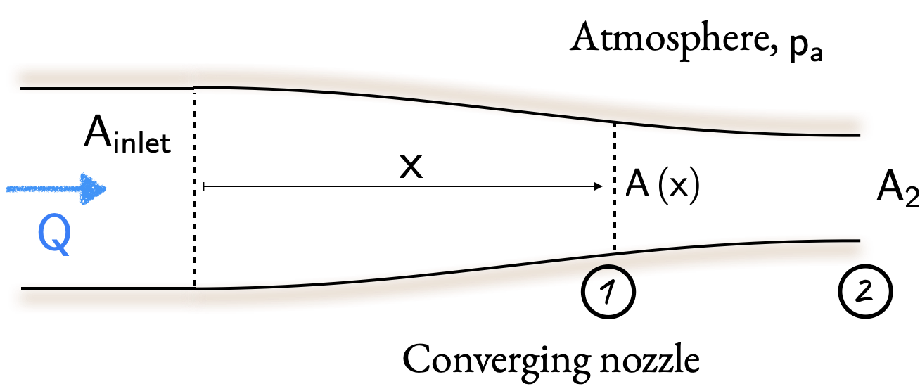
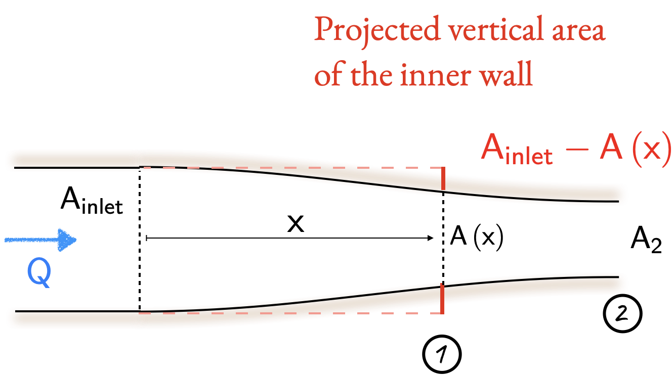
The question states that the nozzle is designed to produce a parallel jet of water. Thus, at the exit we have parallel streamlines and consequently no transverse pressure gradient.

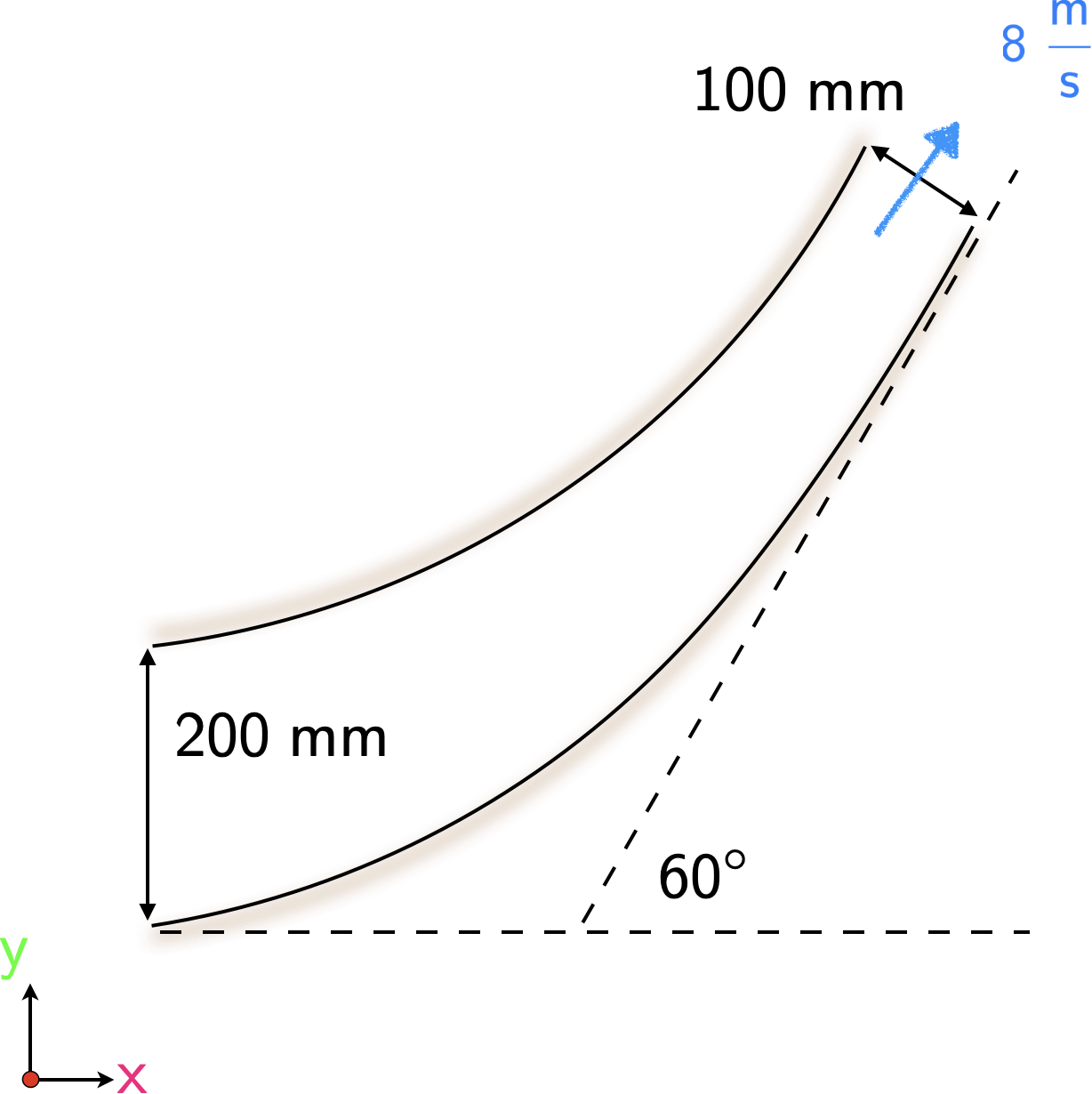
\[ \large \require{color} A_1 = \frac{\pi }{4} \left(0.2\right)^2 = 0.031416 \; m^2, \; \; \; \; \; A_2 = \frac{\pi}{4} \left( 0.1 \right)^2 = 0.007854 \; m^2. \]

The velocity at the entrance can be worked out via continuity. Since we are given no information on the density, we assume the flow is incompressible and therefore the volumetric flow rates are equal. This yields

\[ \large \require{color} A_1 {\color[rgb]{0.059472,0.501943,0.998465}v}_1 = A_2 {\color[rgb]{0.059472,0.501943,0.998465}v}_2 \; \; \; \Rightarrow \; \; \; {\color[rgb]{0.059472,0.501943,0.998465}v}_1 = \frac{A_2 {\color[rgb]{0.059472,0.501943,0.998465}v}_2}{A_1} = \frac{0.1^2 \times {\color[rgb]{0.059472,0.501943,0.998465}8}}{0.2^2} = {\color[rgb]{0.059472,0.501943,0.998465}2 \; m/s}. \]

To work out the massflow rate, we use continuity

\[ \large \require{color} \dot{m} = {\color[rgb]{0.918231,0.469102,0.038229}\rho} A_2 {\color[rgb]{0.059472,0.501943,0.998465}v}_2 = {\color[rgb]{0.918231,0.469102,0.038229}1000} {\color[rgb]{0.918231,0.469102,0.038229} \frac{kg}{m^3}} \times 0.007854 m^2 \times {\color[rgb]{0.059472,0.501943,0.998465}8} {\color[rgb]{0.059472,0.501943,0.998465} \frac{m}{s}} = 62.83 \frac{kg}{s} \]

As this problem makes no statement on pressure losses within the circular nozzle, we can write

\[ \large \require{color} {\color[rgb]{0.315209,0.728565,0.037706}p}_1 + \frac{1}{2}{\color[rgb]{0.918231,0.469102,0.038229}\rho} {\color[rgb]{0.059472,0.501943,0.998465}v}_1^2 = {\color[rgb]{0.315209,0.728565,0.037706}p}_2 + \frac{1}{2}{\color[rgb]{0.918231,0.469102,0.038229}\rho} {\color[rgb]{0.059472,0.501943,0.998465}v}_2^2 \]

\[ \large \require{color} \Rightarrow {\color[rgb]{0.315209,0.728565,0.037706}p}_1 = 0 + \frac{1}{2} {\color[rgb]{0.918231,0.469102,0.038229}\rho} \left( {\color[rgb]{0.059472,0.501943,0.998465}v}_2^2 - {\color[rgb]{0.059472,0.501943,0.998465}v}_1^2\right) \]

\[ \large \require{color} {\color[rgb]{0.315209,0.728565,0.037706}p}_1 = \frac{1}{2} \times 1000 \times \left(8^2 - 2^2\right) = 30 \; kPa \]

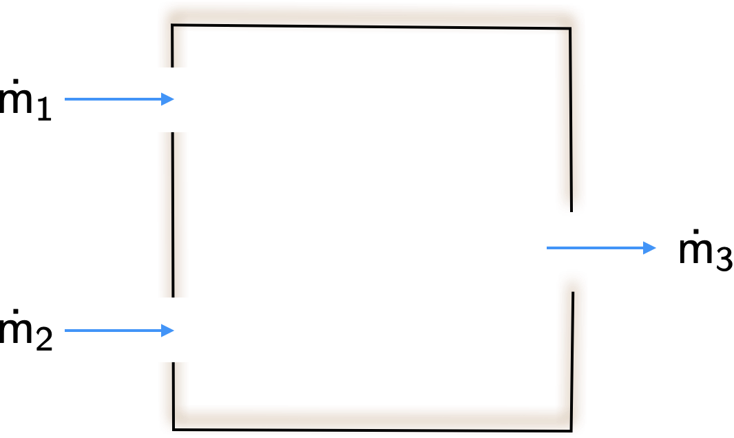
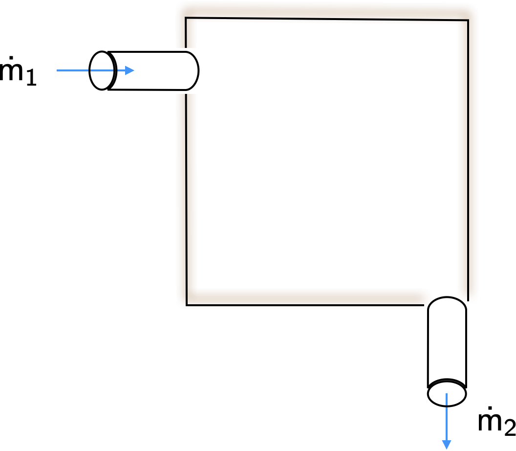
To calculate the forces, consider the diagram below.

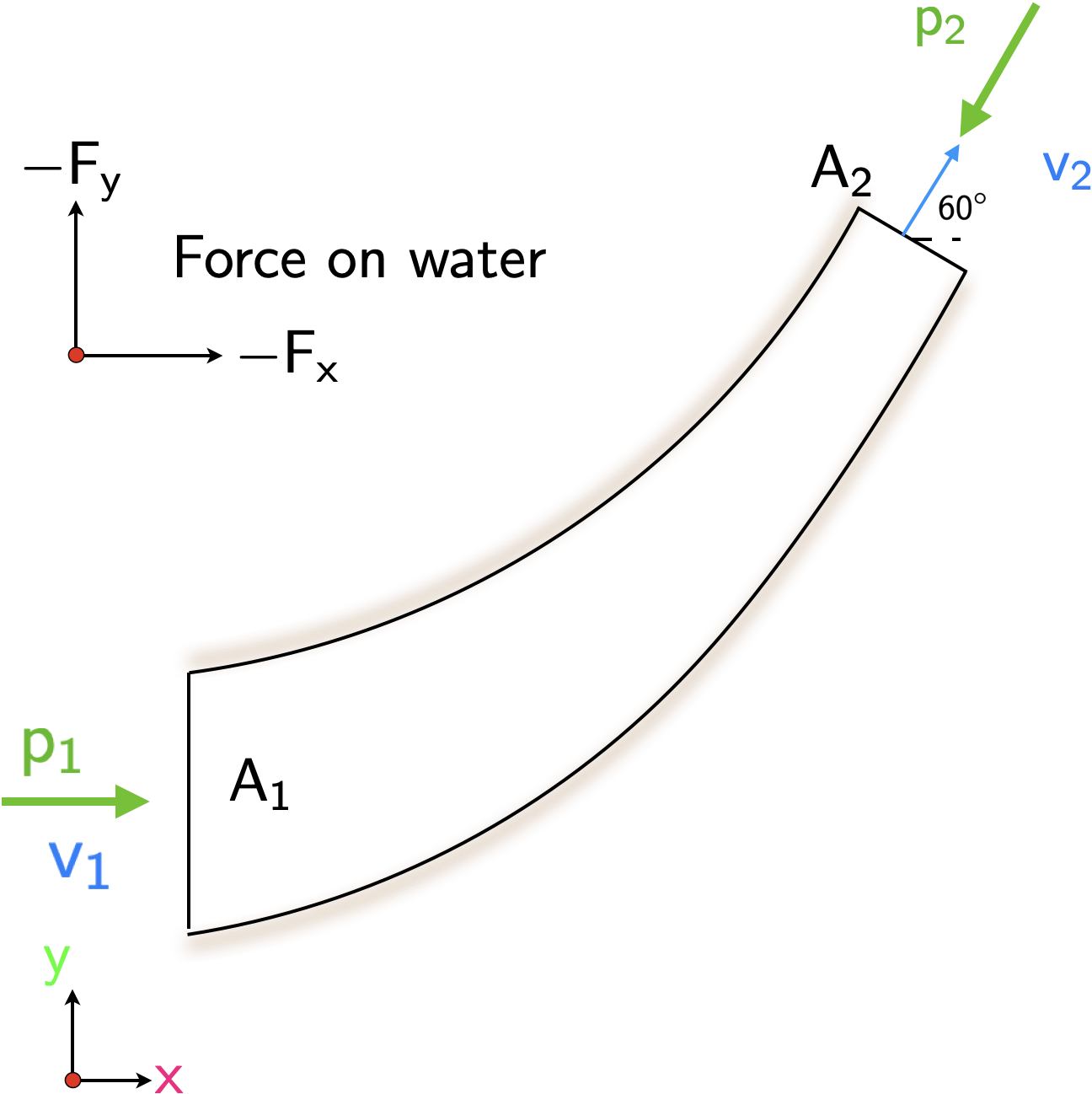
Along the horizontal direction, we have the following steady flow momentum equation

\[ \large \require{color} {\color[rgb]{0.315209,0.728565,0.037706}p}_1 A_1 - F_{x} - {\color[rgb]{0.315209,0.728565,0.037706}p}_2 A_2 cos\left(60^{\circ} \right) = \dot{m} {\color[rgb]{0.059472,0.501943,0.998465}v}_2 cos\left(60^{\circ}\right) - \dot{m} v_1 \]

where we have used the gauge pressure. Along the vertical direction we have

\[ \large \require{color} 0 - F_y - {\color[rgb]{0.315209,0.728565,0.037706}p}_2 A_2 sin\left(60^{\circ}\right) = \dot{m}{\color[rgb]{0.059472,0.501943,0.998465}v}_2 sin\left( 60^{\circ}\right) - 0. \]

Simplifying the above equations individually we have

\[ \large \require{color} F_{x} = \left( {\color[rgb]{0.315209,0.728565,0.037706}p}_1 A_1 - {\color[rgb]{0.315209,0.728565,0.037706}p}_2 A_2 cos\left( 60^{\circ} \right) \right) + \dot{m}\left( {\color[rgb]{0.059472,0.501943,0.998465}v}_1 - {\color[rgb]{0.059472,0.501943,0.998465}v}_2 cos\left(60^{\circ} \right) \right) \]

\[ \large \require{color} \left( 30000 \times 0.031416 - 0 \right) + 62.83 \left(2 - 8 \times 0.5 \right) \]

\[ \large \require{color} 942.48 - 125.66 = 816.82 N \]

and along the vertical direction

\[ \large \require{color} F_y = \left(-{\color[rgb]{0.315209,0.728565,0.037706}p}_2 A_2 sin\left( 60^{\circ}\right) \right) - \dot{m}{\color[rgb]{0.059472,0.501943,0.998465}v}_2 sin\left( 60^{\circ} \right) \]

\[ \large \require{color} 0 - 62.83 \times 8 \times \sqrt{3}/2 = -435.80N \]

Problem 7

The velocity \(\require{color}{\color[rgb]{0.059472,0.501943,0.998465}v}\) at a position \({\color[rgb]{0.986048,0.008333,0.501924}x}\) along the center-line of the convergent entry nozzle of a wind tunnel operating at steady state is given by

\[ \large \require{color} \mathbf{{\color[rgb]{0.059472,0.501943,0.998465}v}} = \left({\color[rgb]{0.059472,0.501943,0.998465}v}_{{\color[rgb]{0.986048,0.008333,0.501924}x}}, {\color[rgb]{0.059472,0.501943,0.998465}v}_{{\color[rgb]{0.131302,0.999697,0.023594}y}}, {\color[rgb]{0.059472,0.501943,0.998465}v}_{{\color[rgb]{0.501963,0.000037,0.250983}z}} \right) \; \; \; \textrm{where} \; \; \; \; {\color[rgb]{0.059472,0.501943,0.998465}v}_{{\color[rgb]{0.986048,0.008333,0.501924}x}} = \alpha\left(0.25 + 0.75 \frac{x}{L} \right), \; {\color[rgb]{0.059472,0.501943,0.998465}v}_{{\color[rgb]{0.131302,0.999697,0.023594}y}}= 0, \; \; \textrm{and} \; \; {\color[rgb]{0.059472,0.501943,0.998465}v}_{{\color[rgb]{0.501963,0.000037,0.250983}z}}=0. \]

The nozzle has length \(\mathsf{L}\) and the velocity in the working section is \(\alpha\).

1. If \(L = 1.2\) m and \(\alpha=10\) m/s, what is the center-line velocity at \(x=0.4\) m?

2. What is the rate of change of the velocity field, \(\partial \mathbf{{\color[rgb]{0.059472,0.501943,0.998465}v}}/\partial t\) at this point? Include the units please.

3. Write down the definition of the material (also known as substantial) derivative, \(D / Dt\), and simplify it for the special case where \({\color[rgb]{0.059472,0.501943,0.998465}v}_{{\color[rgb]{0.131302,0.999697,0.023594}y}}= 0\) and \({\color[rgb]{0.059472,0.501943,0.998465}v}_{{\color[rgb]{0.501963,0.000037,0.250983}z}}= 0\) in Cartesian coordinates. Use this to find the acceleration of a fluid blob as it passes this point. Include the units.

4. Why are your answers to the above two questions different?

Solution

Please find the solutions below:

1. \({\color[rgb]{0.059472,0.501943,0.998465}v}_{{\color[rgb]{0.986048,0.008333,0.501924}x}} = 10 \times (0.25 + 0.75\frac{0.4}{1.2}) = 5 \; \textrm{m}/\textrm{s}\). Note that on the center-line \({\color[rgb]{0.059472,0.501943,0.998465}v}_{{\color[rgb]{0.131302,0.999697,0.023594}y}}\) and \({\color[rgb]{0.059472,0.501943,0.998465}v}_{{\color[rgb]{0.501963,0.000037,0.250983}z}}\) are both zero.

2. The flow is steady so \(\partial \mathbf{{\color[rgb]{0.059472,0.501943,0.998465}v}} / \partial t\) is zero at all points in the flow.

3. The material derivative is defined as:

\[ \large \require{color} \frac{D}{Dt} = \left( \frac{\partial }{\partial t} + \mathbf{{\color[rgb]{0.059472,0.501943,0.998465}v}} \cdot \nabla \right) \]

In the special case where \({\color[rgb]{0.059472,0.501943,0.998465}v}_{{\color[rgb]{0.986048,0.008333,0.501924}x}}\) and \({\color[rgb]{0.059472,0.501943,0.998465}v}_{{\color[rgb]{0.131302,0.999697,0.023594}y}}\) are zero, this reduces to:

\[ \large \require{color} \frac{D}{Dt} = \left( \frac{\partial}{\partial t} + {\color[rgb]{0.059472,0.501943,0.998465}v}_{{\color[rgb]{0.986048,0.008333,0.501924}x}} \frac{\partial}{\partial {\color[rgb]{0.986048,0.008333,0.501924}x}} \right) \]

The acceleration of a fluid blob as it passes this point is given by \(D \mathbf{{\color[rgb]{0.059472,0.501943,0.998465}v}} / Dt\). We know that \({\color[rgb]{0.059472,0.501943,0.998465}v}_{\color[rgb]{0.131302,0.999697,0.023594}y}\) and \({\color[rgb]{0.059472,0.501943,0.998465}v}_{\color[rgb]{0.501963,0.000037,0.250983}z}\) are both zero, so this reduces to \(D{\color[rgb]{0.059472,0.501943,0.998465}v}_{{\color[rgb]{0.986048,0.008333,0.501924}x}} / Dt\):

\[ \large \require{color} \frac{D {\color[rgb]{0.059472,0.501943,0.998465}v}_{{\color[rgb]{0.986048,0.008333,0.501924}x}}}{Dt} = 0 + {\color[rgb]{0.059472,0.501943,0.998465}v}_{{\color[rgb]{0.986048,0.008333,0.501924}x}} \frac{0.75 \alpha}{L} = 5 \times \frac{0.75 \times 10}{1.2} = 31.25 \frac{m}{s^2}. \]

4. Although the flow is steady at all points in space, fluid blobs do accelerate as the move through the flow field. This is the main point of the question.