L16 examples

Problem 1

A gas-powered refrigerator works by taking in heat from a heat exchanger at $500^{\circ} C$ and from a cold space at $- 10^{\circ} C$ , while rejecting heat to the environment at $35^{\circ} C$ . The refrigerator is a cyclic device, and there is no work input or output. Use the Clausius inequality to find the minimum rate at which heat must be supplied by the heat exchanger in order to extract heat at a rate of $1 k W$ from the cold space.

Solution

This problem is very similar to the one covered in Lecture 16. It will be useful to consider the diagram below.

cycle

From the 1st law we have:

${\dot{Q}}_{1} + {\dot{Q}}_{2} = {\dot{Q}}_{3}$

and from the second law (the Clausius inequality):

$\sum \frac{{\dot{Q}}_{i}}{T_{i}} \leq 0$

As noted in Lecture 16, the minus sign sign that preceeds ${\dot{Q}}_{3}$ denotes it is going out of the system. Eliminating ${\dot{Q}}_{3}$ from the two expressions yields:

$\frac{{\dot{Q}}_{1}}{T_{1}} + \frac{{\dot{Q}}_{2}}{T_{2}} - \frac{({\dot{Q}}_{1} + {\dot{Q}}_{2})}{T_{3}} \leq 0$

Rearranging the above gives

$\frac{{\dot{Q}}_{1}}{{\dot{Q}}_{2}} \geq (\frac{1 / T_{2} - 1 / T_{3}}{1 / T_{3} - 1 / T_{1}})$

with the numerical solution given below.

Code

import numpy as np

absolute_zero = 273.15 
T_1 = 500 + absolute_zero # all in Kelvin!
T_2 = -10 + absolute_zero
T_3 = 35 + absolute_zero
dot_Q1_by_dot_Q2 = (1./T_2 - 1./T_3)/(1./T_3 - 1./T_1)
dot_Q2 = 1 # kW
dot_Q1 = dot_Q1_by_dot_Q2 * dot_Q2
print('The minimum heat supply rate from the heat exchanger (source) is '+str(np.round(dot_Q1, 3))+' kW')

The minimum heat supply rate from the heat exchanger (source) is 0.284 kW

Problem 2

A cyclic heat pump takes $600 M J$ (mega joules) of heat at $27^{\circ} C$ while rejecting heat to a system whose temperature rises $1^{\circ} C$ for each MJ of energy supplied to it. Initially this system is also at $27^{\circ} C$ .

Explain why there is a limit on the final temperature of the system. State whether it is an upper or lower limit, and under what circumstances it would be reached.
Calculate the limit on the final temperature of the system. What is the work input to the heat pump when this limit is achieved?

Solution

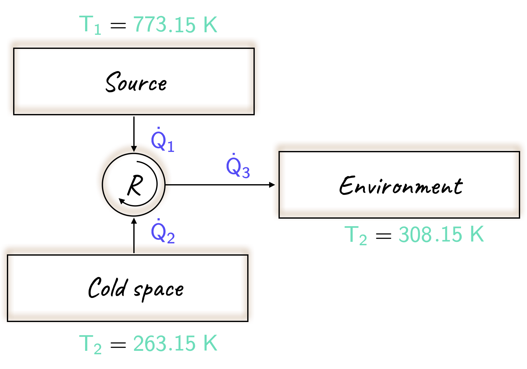
As before, it will be useful to sketch out a diagram of the process above.

cycle

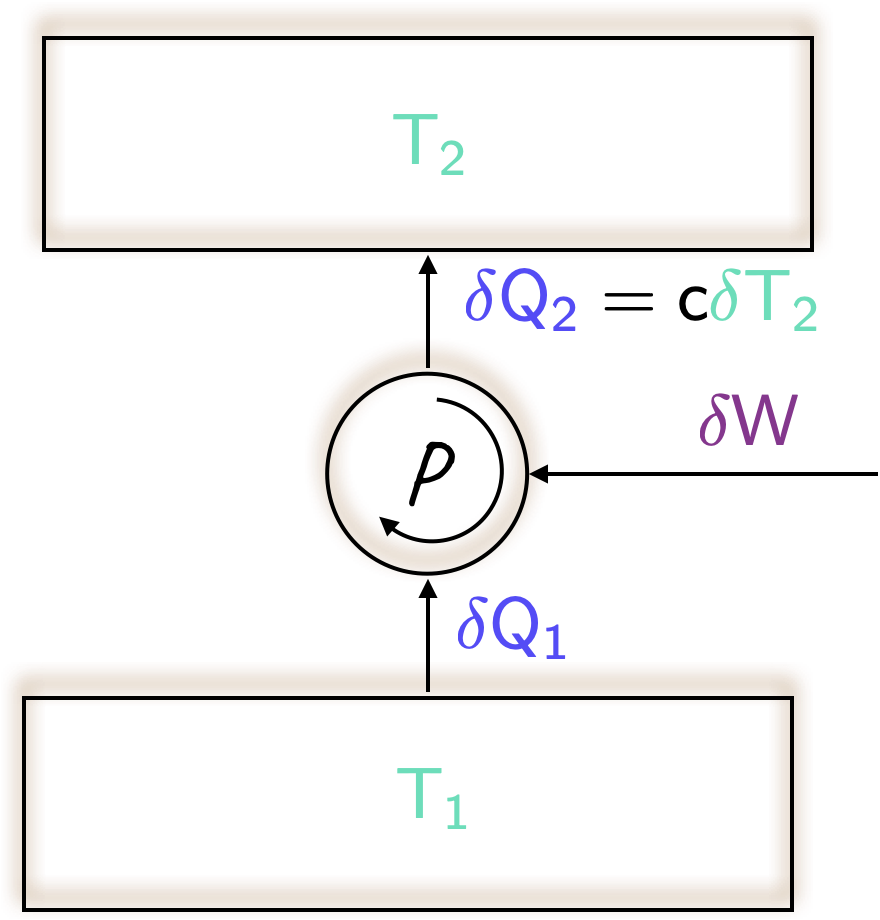
From the first law, it is clear that

$δ Q_{2} = δ Q_{1} + δ W .$

Note that if the pump were reversible, then it would be as efficient as possible, implying that the amount of work $δ W$ required by the pump would be as low as possible. This sets a lower limit on work, which consequently also sets a lower limit on $δ Q_{2}$ , and therefore on $T_{2}$ .

Consider the Clausius statement (with appropriate signs)

$\frac{δ Q_{1}}{T_{1}} - \frac{δ Q_{2}}{T_{2}} \leq 0$

From the problem statement, we can infer that the constant $c = 1 M J / K$ , leading to

$\frac{c δ T_{2}}{T_{2}} \geq \frac{δ Q_{1}}{T_{1}} .$

Integrating both sides of this equation

$\int_{300}^{T_{f}} \frac{c δ T_{2}}{T_{2}} \geq \frac{Q_{1}}{T_{1}}$

$\Rightarrow 1 \times l n (\frac{T_{f}}{300.15}) \geq \frac{600}{300.15} \Rightarrow T_{f} \geq 2217.82 K$

Note that for the reversible case

$Q_{2} = (2217.82 - 300.15) / c = 1917.67 M J$

Thus the work input is

$W = 1917.67 - 600 = 1316.7 M J$ .