Problem 1

Water with a density of \(\require{color}{\color[rgb]{0.990448,0.502245,0.032881}1000 \frac{kg}{m^3}}\) is ejected from a fire-hose at \(20\; m/s\). The gauge pressure inside the fire-hose is \(1.9 \times 10^{5} \; N/m^2\). Assume the fire-hose has a circular cross-section throughout. Calculate the force required to hold the fire-hose, negating any height varying pressure force. Consider the free-body diagram given below.

View of a fire-hose Free-body diagram
channel orifice

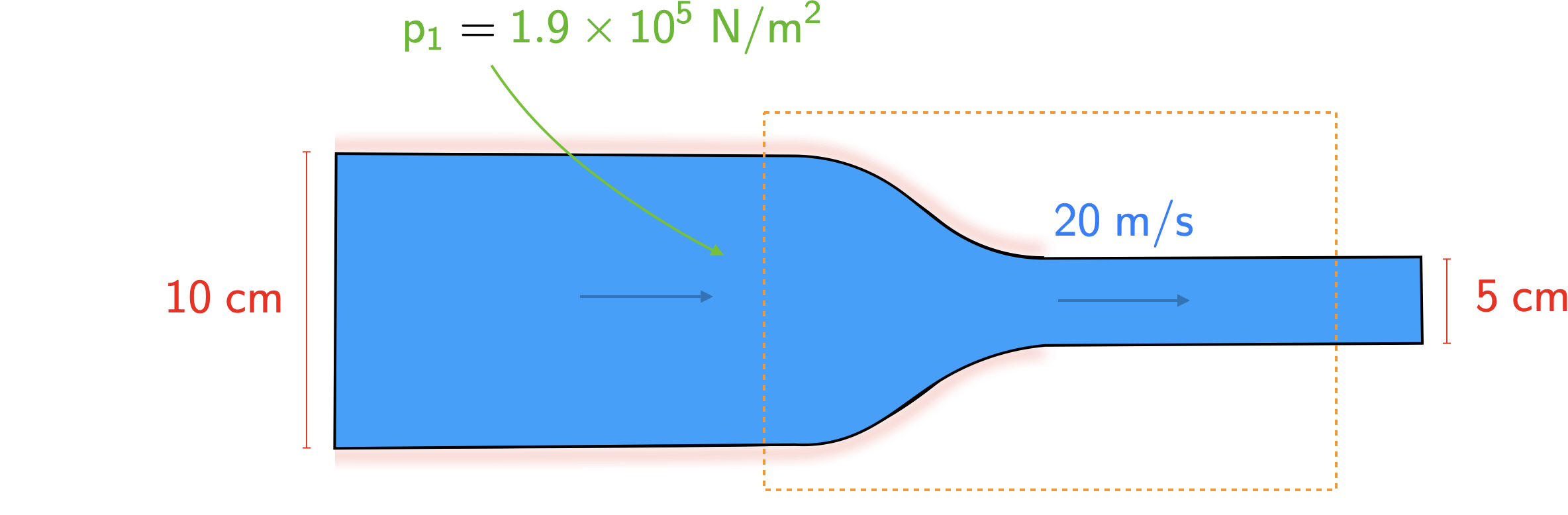
Note the control volume that has been drawn around the nozzle.

Solution

On the left-hand side, we have both \(\require{color}{\color[rgb]{0.315209,0.728565,0.037706}p_1}\) and atmoshpheric pressure acting, while on the right-hand side it is just atmospheric pressure. Thus, we can express the pressure forces as:

\[ \large \require{color}\sum {\color[rgb]{0.315209,0.728565,0.037706}p}A = {\color[rgb]{0.315209,0.728565,0.037706}p_1} A_1 - 0. \]

Applying the steady flow momentum equation along the horizontal direction yields

\[ \large \require{color}F_{\color[rgb]{0.986048,0.008333,0.501924}x} + \sum {\color[rgb]{0.315209,0.728565,0.037706}p}A = \sum \dot{m}_{out} {\color[rgb]{0.059472,0.501943,0.998465}v_{out}} - \sum \dot{m}_{in} {\color[rgb]{0.059472,0.501943,0.998465}v_{in} }. \]

From continuity, we now that \(\dot{m}_{out} = \dot{m}_{in}\), leading to

\[ \large \require{color}F_{\color[rgb]{0.986048,0.008333,0.501924}x} + {\color[rgb]{0.315209,0.728565,0.037706}p_1}A_1 =\dot{m}_{in} \left( {\color[rgb]{0.059472,0.501943,0.998465}v_{out}} - {\color[rgb]{0.059472,0.501943,0.998465}v_{in} } \right) \]

\[ \large \require{color}F_{\color[rgb]{0.986048,0.008333,0.501924}x} + {\color[rgb]{0.315209,0.728565,0.037706}p_1}A_1 = {\color[rgb]{0.918231,0.469102,0.038229}\rho} A_{in} {\color[rgb]{0.059472,0.501943,0.998465}v_{in} }\left( {\color[rgb]{0.059472,0.501943,0.998465}v_{out}} - {\color[rgb]{0.059472,0.501943,0.998465}v_{in} } \right) \]

\[ \large \require{color}F_{\color[rgb]{0.986048,0.008333,0.501924}x} = {\color[rgb]{0.918231,0.469102,0.038229}\rho} A_{in} {\color[rgb]{0.059472,0.501943,0.998465}v_{in} }\left( {\color[rgb]{0.059472,0.501943,0.998465}v_{out}} - {\color[rgb]{0.059472,0.501943,0.998465}v_{in} } \right) - {\color[rgb]{0.315209,0.728565,0.037706}p_1}A_1. \]

Next we work out the velocity at the inflow using continuity, i.e., \(\dot{m}_{in} = \dot{m}_{out}\),

\[ \large \require{color}{\color[rgb]{0.059472,0.501943,0.998465}v_{in}} = \frac{A_{out}}{A_{in}} {\color[rgb]{0.059472,0.501943,0.998465}v_{out}} = \left( \frac{5m}{10m} \right)^2 \; {\color[rgb]{0.059472,0.501943,0.998465}20 m/s} = {\color[rgb]{0.059472,0.501943,0.998465}5 m/s}. \]

Plugging in the velocity values, we have \[ \large \require{color}F_{\color[rgb]{0.986048,0.008333,0.501924}x} = {\color[rgb]{0.990448,0.502245,0.032881}1000 \frac{kg}{m^3}} \frac{\pi}{4} \left( 0.1 m \right)^2 {\color[rgb]{0.059472,0.501943,0.998465}5 m/s }\left( {\color[rgb]{0.059472,0.501943,0.998465}20 m/s} - {\color[rgb]{0.059472,0.501943,0.998465}5 m/s } \right) - {\color[rgb]{0.315209,0.728565,0.037706}p_1}\frac{\pi}{4} \left( 0.1 m \right)^2. \]

For numerical values, please see the code below.
Code
import numpy as np

rho = 1000 # kg/m^3
p_1 = 1.9 * 10**5 # N/m^2 
A_in = np.pi/4 * 0.1**2 # m^2
A_out = np.pi/4 * 0.05**2 # m^2
v_out = 20 # m/s
v_in = (A_out / A_in) * v_out
F_x = rho * A_in * v_in * (v_out - v_in) - p_1 * A_in
print(str(F_x)+' N')
-903.2078879070656 N

Problem 2

Let us re-visit the first problem from Lecture 3. We want to calculcate the momentum flux of fluid moving through a pipe with a parabolic velocity profile given by

\[ \large \require{color}{\color[rgb]{0.059472,0.501943,0.998465}v} \left( r \right) = V_o \left( 1 - \left( \frac{r}{{\color[rgb]{0.501967,0.001556,0.998511}R}} \right)^2 \right). \]

The radius \(\require{color}{\color[rgb]{0.501967,0.001556,0.998511}R} = 1 \; m\), and the density of the fluid in the pipe is \(\require{color}{\color[rgb]{0.964810,0.470942,0.057578}\rho} = \require{color}{\color[rgb]{0.964810,0.470942,0.057578}1000 kg / m^3}\), and the constant \(V_o = 10\).

reservoir

Solution

As before, it will be useful to consider a ring-shaped element for the area; see the diagram below.

reservoir

The massflow rate is given by

\[ \large \require{color}\dot{m} {\color[rgb]{0.059472,0.501943,0.998465}v} = \int_{{\color[rgb]{0.064095,0.501831,0.501977}A}} {\color[rgb]{0.990448,0.502245,0.032881}\rho} {\color[rgb]{0.059472,0.501943,0.998465}v}^2 {\color[rgb]{0.064095,0.501831,0.501977}dA} \]

From the diagram above, we can use the following statement

\[ \large \require{color}{\color[rgb]{0.064095,0.501831,0.501977}dA} = 2 \pi r dr. \]

This can then be substituted back into the equation for the massflow rate to yield

\[ \large \require{color}\dot{m}{\color[rgb]{0.059472,0.501943,0.998465}v} = \int_{0}^{{\color[rgb]{0.501967,0.001556,0.998511}R}} {\color[rgb]{0.990448,0.502245,0.032881}\rho} {\color[rgb]{0.059472,0.501943,0.998465}v}^2 \left(r \right) 2 \pi r dr \]

Integrating this out yields

\[ \large \require{color}\dot{m} {\color[rgb]{0.059472,0.501943,0.998465}v}= \int_{0}^{{\color[rgb]{0.501967,0.001556,0.998511}R}} {\color[rgb]{0.990448,0.502245,0.032881}\rho} V^2_o \left( 1 - \left( \frac{r}{{\color[rgb]{0.501967,0.001556,0.998511}R}} \right)^2 \right)^2 2 \pi r dr \]

\[ \large \require{color}\dot{m} {\color[rgb]{0.059472,0.501943,0.998465}v}= 2 \pi {\color[rgb]{0.990448,0.502245,0.032881}\rho} V^2_o \int_{0}^{{\color[rgb]{0.501967,0.001556,0.998511}R}} \left( 1 - \left( \frac{r}{{\color[rgb]{0.501967,0.001556,0.998511}R}} \right)^2 \right)^2 r dr \]

\[ \large \require{color}\dot{m}{\color[rgb]{0.059472,0.501943,0.998465}v} = 2 \pi {\color[rgb]{0.990448,0.502245,0.032881}\rho} V^2_o \int_{0}^{{\color[rgb]{0.501967,0.001556,0.998511}R}} \left( r - \frac{2r^3}{{\color[rgb]{0.501967,0.001556,0.998511}R}^2} + \frac{r^5}{{\color[rgb]{0.501967,0.001556,0.998511}R}^4} \right) dr \]

\[ \large \require{color}\dot{m} {\color[rgb]{0.059472,0.501943,0.998465}v}= 2 \pi {\color[rgb]{0.990448,0.502245,0.032881}\rho} V^2_o \left[ \frac{{\color[rgb]{0.501967,0.001556,0.998511}R}^2}{2} - \frac{2{\color[rgb]{0.501967,0.001556,0.998511}R}^2}{4} + \frac{{\color[rgb]{0.501967,0.001556,0.998511}R}^2}{6} - 0\right] \]

\[ \large \require{color}\dot{m} {\color[rgb]{0.059472,0.501943,0.998465}v}= 2 \pi {\color[rgb]{0.990448,0.502245,0.032881}\rho} V^2_o \frac{{\color[rgb]{0.501967,0.001556,0.998511}R^2}}{6} = \frac{\pi}{3}{\color[rgb]{0.990448,0.502245,0.032881}\rho} V^2_o {\color[rgb]{0.501967,0.001556,0.998511}R^2} \]

It is worth noting that the solution above is simply not the solution from Lecture 3 multiplied by the mean velocity \(V_0/2\) ! In other words, one has to work through the integrals. Given the formula above, we can now calculate the momentum flux.
Code
V_o = 10
rho = 1000
R = 1
mdot_v = 1./3 * np.pi * rho * V_o**2 * R**2 
print(str(mdot_v/1000)+' kN')
104.71975511965978 kN