Code
import numpy as np

m = 0.130
T_2 = 600 + 273.15
T_1 = 950 + 273.15
alpha = 555.65
beta = 0.392

W = m * (alpha * (T_1 - T_2) + 0.5 * beta * (T_1**2 - T_2**2))
print('Work done is '+str(np.round(W/1000, 3))+' kJ')
Work done is 43.977 kJCarbon dioxide (with a molar mass of \(44 \; g/mol\)) behaves like a semi-perfect gas at moderate pressures and temperatures. Over the temperature range \(\require{color}{\color[rgb]{0.164799,0.878862,0.723179}500^{\circ} \; C}\) to \(\require{color}{\color[rgb]{0.164799,0.878862,0.723179}1200^{\circ} \; C}\), its constant volume specific heat capacity is accurately represented by the linear relation:
\[ \large \require{color} {\color[rgb]{0.878548,0.880173,0.060757}c}_{\color[rgb]{0.079785,0.618358,0.483717}V} = \alpha + \beta {\color[rgb]{0.164799,0.878862,0.723179}T} \]
where \(\alpha=555.65 \; J / \left( kg \cdot K \right)\) and \(\beta = 0.392 \; J / \left( kg \cdot K^2 \right)\). Please note that in the expression above \(\require{color}{\color[rgb]{0.164799,0.878862,0.723179}T}\) is in units Kelvin. A quantity of carbon dioxide undergoes a fully resisted expansion in an insulated cylinder. The initial pressure, volume, and temperature are \({\color[rgb]{0.315209,0.728565,0.037706}0.3 \; MPa}\), \({\color[rgb]{0.079785,0.618358,0.483717}0.1 \; m^3}\) and \({\color[rgb]{0.164799,0.878862,0.723179}950^{\circ} \; C}\) respectively. At the end of the expansion the temperature has fallen to \({\color[rgb]{0.164799,0.878862,0.723179}600^{\circ} \; C}\). You will need the universal gas constant value of \(8.3145 \; J / \left( mol \cdot K \right)\).
Calculate the mass of carbon dioxide in the cylinder.
Is the relationship \(\require{color}{\color[rgb]{0.315209,0.728565,0.037706}p}{\color[rgb]{0.079785,0.618358,0.483717}V}^{\gamma} = constant\) valid for this process?
Calculate the final volume and pressure.
Determine the work done during the expansion.
\[ \large \require{color} m = \frac{{\color[rgb]{0.315209,0.728565,0.037706}p}V}{ R{\color[rgb]{0.164799,0.878862,0.723179}T}} \]
where for carbon dioxide we have
\[ \large R = \frac{8.3145 \; \frac{J}{mol \cdot K}}{44 \; \frac{g}{mol}} = 0.18896 \frac{J}{g \cdot K} \times \frac{1000 \; g }{kg} = 189 \frac{J}{kg \cdot K}. \]
Please note that for both perfect and semi-perfect gases, the ideal gas equation is valid. Thus the mass is given by
\[ \large \require{color} m = {\color[rgb]{0.315209,0.728565,0.037706}0.3 \times 10^6} \times \frac{{\color[rgb]{0.079785,0.618358,0.483717}0.1}}{189 \times \left({\color[rgb]{0.164799,0.878862,0.723179} 950 + 273.15}\right) }=0.130 \; kg \]
No the relationship is not constant because this is not a perfect gas (where \(\require{color}{\color[rgb]{0.878548,0.880173,0.060757}c}_{\color[rgb]{0.079785,0.618358,0.483717}V}\) is a constant).
The first law per unit mass (using specific quantities) is given by
\[ \large \require{color} {\color[rgb]{0.334690,0.296180,0.998454}dq} - {\color[rgb]{0.562040,0.190215,0.568721}dw} = {\color[rgb]{0.878548,0.880173,0.060757}du} \]
As the cylinder is given to be fully insulated, we assume an adiabatic process, i.e., \(\require{color}{\color[rgb]{0.334690,0.296180,0.998454}dq} = 0\). Additionally as its fully resisted, we have
\[ \large \require{color} {\color[rgb]{0.562040,0.190215,0.568721}dw} = {\color[rgb]{0.315209,0.728565,0.037706}p} {\color[rgb]{0.918231,0.469102,0.038229}d \nu} \]
where \(\require{color}{\color[rgb]{0.918231,0.469102,0.038229}\nu}\) is the specific volume. From these relationships we arrive at
\[ \large \require{color} {\color[rgb]{0.315209,0.728565,0.037706}p} {\color[rgb]{0.918231,0.469102,0.038229}d \nu} + {\color[rgb]{0.878548,0.880173,0.060757}du} = 0 \]
Recognizing that the internal energy is specific and using the definition of an ideal gas we have
\[ \large \require{color} R{\color[rgb]{0.164799,0.878862,0.723179}T}\frac{{\color[rgb]{0.918231,0.469102,0.038229}d\nu}}{{\color[rgb]{0.918231,0.469102,0.038229}\nu}} + {\color[rgb]{0.878548,0.880173,0.060757}c}_{{\color[rgb]{0.079785,0.618358,0.483717}V}} {\color[rgb]{0.164799,0.878862,0.723179}dT} = 0 \]
\[ \large \require{color} \Rightarrow R{\color[rgb]{0.164799,0.878862,0.723179}T}\frac{{\color[rgb]{0.918231,0.469102,0.038229}d\nu}}{{\color[rgb]{0.918231,0.469102,0.038229}\nu}} + \left( \alpha + \beta {\color[rgb]{0.164799,0.878862,0.723179}T} \right) {\color[rgb]{0.164799,0.878862,0.723179}dT} = 0 \]
\[ \large \require{color} \Rightarrow R{\color[rgb]{0.164799,0.878862,0.723179}T}\frac{{\color[rgb]{0.918231,0.469102,0.038229}d\nu}}{{\color[rgb]{0.918231,0.469102,0.038229}\nu}} + \alpha {\color[rgb]{0.164799,0.878862,0.723179}dT}+ \beta {\color[rgb]{0.164799,0.878862,0.723179}T} {\color[rgb]{0.164799,0.878862,0.723179}dT} = 0 \]
\[ \large \require{color} \Rightarrow R \frac{{\color[rgb]{0.918231,0.469102,0.038229}d\nu}}{{\color[rgb]{0.918231,0.469102,0.038229}\nu}} + \frac{\alpha}{{\color[rgb]{0.164799,0.878862,0.723179}T}} {\color[rgb]{0.164799,0.878862,0.723179}dT}+ \beta {\color[rgb]{0.164799,0.878862,0.723179}dT} = 0 \]
Now integrating between states 1 and 2 yields
\[ \large \require{color} R \; ln \left( \frac{{\color[rgb]{0.918231,0.469102,0.038229}\nu_2}}{{\color[rgb]{0.918231,0.469102,0.038229}\nu_1}} \right) = \alpha \; ln \left( \frac{{\color[rgb]{0.164799,0.878862,0.723179}T_1}}{{\color[rgb]{0.164799,0.878862,0.723179}T_2}} \right) + \beta \left({\color[rgb]{0.164799,0.878862,0.723179}T_1} - {\color[rgb]{0.164799,0.878862,0.723179}T_2} \right) \]
\[ \large \require{color} \Rightarrow ln \left( \frac{{\color[rgb]{0.079785,0.618358,0.483717}V_2}}{{\color[rgb]{0.079785,0.618358,0.483717}V_1}} \right) = ln \left( \frac{{\color[rgb]{0.918231,0.469102,0.038229}\nu_2}}{{\color[rgb]{0.918231,0.469102,0.038229}\nu_1}} \right) = \frac{\alpha}{R} ln \left( \frac{{\color[rgb]{0.164799,0.878862,0.723179}T_1}}{{\color[rgb]{0.164799,0.878862,0.723179}T_2}} \right) + \frac{\beta}{R} \left({\color[rgb]{0.164799,0.878862,0.723179}T_1} - {\color[rgb]{0.164799,0.878862,0.723179}T_2} \right) \]
\[ \large \require{color} = \frac{555.65}{189} \; ln \left(\frac{{\color[rgb]{0.164799,0.878862,0.723179}1223.15}}{{\color[rgb]{0.164799,0.878862,0.723179}873.15}} \right) + \frac{0.392}{189} \left({\color[rgb]{0.164799,0.878862,0.723179}1223.15} - {\color[rgb]{0.164799,0.878862,0.723179}873.15} \right) \]
This leads to
\[ \large \require{color} {\color[rgb]{0.079785,0.618358,0.483717}V_2} = 5.567 {\color[rgb]{0.079785,0.618358,0.483717}V_1} \Rightarrow {\color[rgb]{0.079785,0.618358,0.483717}V_2} = {\color[rgb]{0.079785,0.618358,0.483717}0.557 \; m^3} \]
Now we can work out the final pressure, i.e.,
\[ \large \require{color} {\color[rgb]{0.315209,0.728565,0.037706}p_2} = \frac{mR{\color[rgb]{0.164799,0.878862,0.723179}T_2}}{{\color[rgb]{0.079785,0.618358,0.483717}V_2}} = \frac{0.130 \times 189 \times {\color[rgb]{0.164799,0.878862,0.723179}873.15}}{{\color[rgb]{0.079785,0.618358,0.483717}0.557}} = {\color[rgb]{0.315209,0.728565,0.037706}38.50 \; kPa} \]
\[ \require{color} \large {\color[rgb]{0.562040,0.190215,0.568721}W }= -{\color[rgb]{0.878548,0.880173,0.060757}\Delta U} = - m \int_{1}^{2} {\color[rgb]{0.878548,0.880173,0.060757}c}_{\color[rgb]{0.079785,0.618358,0.483717}V} {\color[rgb]{0.164799,0.878862,0.723179}dT} = m \int_{2}^{1} {\color[rgb]{0.878548,0.880173,0.060757}c}_{\color[rgb]{0.079785,0.618358,0.483717}V} {\color[rgb]{0.164799,0.878862,0.723179}dT} = m \left[ \alpha \left( {\color[rgb]{0.164799,0.878862,0.723179}T_1} - {\color[rgb]{0.164799,0.878862,0.723179}T_2} \right) + \frac{1}{2} \beta \left( {\color[rgb]{0.164799,0.878862,0.723179}T_1}^2 - {\color[rgb]{0.164799,0.878862,0.723179}T_2}^2 \right) \right]. \]
The numerical solution is given below
import numpy as np
m = 0.130
T_2 = 600 + 273.15
T_1 = 950 + 273.15
alpha = 555.65
beta = 0.392
W = m * (alpha * (T_1 - T_2) + 0.5 * beta * (T_1**2 - T_2**2))
print('Work done is '+str(np.round(W/1000, 3))+' kJ')Work done is 43.977 kJA quantity of argon gas with \(\gamma = 1.67\), initially at \(\require{color}{\color[rgb]{0.315209,0.728565,0.037706}1 \; bar}\) and \(\require{color}{\color[rgb]{0.164799,0.878862,0.723179}300 \; K}\) is compressed adiabatically and reversibly (and hence isentropically) to half its initial volume. Calculate the final pressure and temperature.
As the question states, the process is isentropic. We can make use of the isentropic relations presented in Lecture 14, i.e.,
\[ \large \require{color} \frac{{\color[rgb]{0.315209,0.728565,0.037706}p_2}}{{\color[rgb]{0.315209,0.728565,0.037706}p_1}} = \left( \frac{{\color[rgb]{0.164799,0.878862,0.723179}V_1}}{{\color[rgb]{0.164799,0.878862,0.723179}V_2}} \right)^{\gamma} \Rightarrow {\color[rgb]{0.315209,0.728565,0.037706}p_2} = {\color[rgb]{0.315209,0.728565,0.037706}p_1} \left( \frac{{\color[rgb]{0.164799,0.878862,0.723179}V_1}}{{\color[rgb]{0.164799,0.878862,0.723179}V_2}} \right)^{\gamma} = {\color[rgb]{0.315209,0.728565,0.037706}1} \times {\color[rgb]{0.079785,0.618358,0.483717}2}^{1.67} = {\color[rgb]{0.315209,0.728565,0.037706}3.18 \; bar} \]
and for the temperature, we have
\[ \large \require{color} {\color[rgb]{0.164799,0.878862,0.723179}T_2} = {\color[rgb]{0.164799,0.878862,0.723179}T_1} \left( \frac{{\color[rgb]{0.079785,0.618358,0.483717}V_1}}{{\color[rgb]{0.079785,0.618358,0.483717}V_2}} \right)^{\gamma - 1} = {\color[rgb]{0.164799,0.878862,0.723179}300} \times {\color[rgb]{0.079785,0.618358,0.483717}2}^{0.67} = {\color[rgb]{0.164799,0.878862,0.723179}477.3 \; K} \]
A polytropic process is defined by the relation
\[ \large \require{color}{\color[rgb]{0.315209,0.728565,0.037706}p}{\color[rgb]{0.079785,0.618358,0.483717}V}^{n} = k \]
where \(n\) and \(k\) are constants.
\[ \large \require{color}{\color[rgb]{0.562040,0.190215,0.568721}W} = \frac{{\color[rgb]{0.315209,0.728565,0.037706}p_1} {\color[rgb]{0.079785,0.618358,0.483717}V_1} - {\color[rgb]{0.315209,0.728565,0.037706}p_2} {\color[rgb]{0.079785,0.618358,0.483717}V_2}}{n-1} \]
provided \(1 \neq n\).
\[ \large \require{color}\frac{{\color[rgb]{0.334690,0.296180,0.998454}Q}}{{\color[rgb]{0.562040,0.190215,0.568721}W}} = \frac{\gamma - n}{\gamma - 1} \]
\[ \large \require{color} {\color[rgb]{0.562040,0.190215,0.568721}W} = \int {\color[rgb]{0.315209,0.728565,0.037706}p} \; {\color[rgb]{0.079785,0.618358,0.483717}dV} = \int_{1}^{2} \frac{k}{{\color[rgb]{0.079785,0.618358,0.483717}V}^n} {\color[rgb]{0.079785,0.618358,0.483717}dV} = k \left[ \frac{{\color[rgb]{0.079785,0.618358,0.483717}V}^{1-n}}{1-n} \right]_{1}^{2} = \frac{{\color[rgb]{0.315209,0.728565,0.037706}p_1} {\color[rgb]{0.079785,0.618358,0.483717}V_1} - {\color[rgb]{0.315209,0.728565,0.037706}p_2} {\color[rgb]{0.079785,0.618358,0.483717}V_2}}{n-1} \]
since \(\require{color}k = {\color[rgb]{0.315209,0.728565,0.037706}p_1} {\color[rgb]{0.079785,0.618358,0.483717}V_1}^{n} = {\color[rgb]{0.315209,0.728565,0.037706}p_2} {\color[rgb]{0.079785,0.618358,0.483717}V_2}^{n}\).
\[ \large \require{color} {\color[rgb]{0.562040,0.190215,0.568721}W} = \frac{{\color[rgb]{0.315209,0.728565,0.037706}p_1} {\color[rgb]{0.079785,0.618358,0.483717}V_1} - {\color[rgb]{0.315209,0.728565,0.037706}p_2} {\color[rgb]{0.079785,0.618358,0.483717}V_2}}{n-1} = mR \frac{\left({\color[rgb]{0.164799,0.878862,0.723179}T_1} - {\color[rgb]{0.164799,0.878862,0.723179}T_2}\right)}{n-1} \]
\[ \large \require{color} {\color[rgb]{0.878548,0.880173,0.060757}\Delta U} = m {\color[rgb]{0.878548,0.880173,0.060757}c}_{\color[rgb]{0.079785,0.618358,0.483717}V} \left({\color[rgb]{0.164799,0.878862,0.723179}T_2} - {\color[rgb]{0.164799,0.878862,0.723179}T_1} \right) = m R \frac{\left( {\color[rgb]{0.164799,0.878862,0.723179}T_2} - {\color[rgb]{0.164799,0.878862,0.723179}T_1} \right) }{\left(\gamma - 1\right) } \]
This yields
\[ \large \require{color} {\color[rgb]{0.334690,0.296180,0.998454}Q} = {\color[rgb]{0.878548,0.880173,0.060757}\Delta U} + {\color[rgb]{0.562040,0.190215,0.568721}W} = m R \left({\color[rgb]{0.164799,0.878862,0.723179}T_1} - {\color[rgb]{0.164799,0.878862,0.723179}T_2} \right) \left[ \frac{1}{n-1} - \frac{1}{\gamma - 1} \right] \]
Thus
\[ \large \require{color} \frac{{\color[rgb]{0.334690,0.296180,0.998454}Q}}{{\color[rgb]{0.562040,0.190215,0.568721}W}} = \left[ \frac{1}{n-1} - \frac{1}{\gamma-1} \right] \left(n - 1 \right) = \frac{\gamma - n}{\gamma - 1} \]
Starting from the first law of Thermodynamics and the definition of entropy
\[ \large \require{color} {\color[rgb]{0.164799,0.878862,0.723179}T} {\color[rgb]{0.599997,0.600015,0.600005}ds} = {\color[rgb]{0.878548,0.880173,0.060757}du} + {\color[rgb]{0.315209,0.728565,0.037706}p} {\color[rgb]{0.918231,0.469102,0.038229}d \nu} \]
\[ \large \require{color} {\color[rgb]{0.164799,0.878862,0.723179}T} {\color[rgb]{0.599997,0.600015,0.600005}ds} = {\color[rgb]{0.986252,0.007236,0.027423}dh} - {\color[rgb]{0.918231,0.469102,0.038229}\nu} {\color[rgb]{0.315209,0.728565,0.037706}dp} \]
\[ \large \require{color} {\color[rgb]{0.599997,0.600015,0.600005}s_2} - {\color[rgb]{0.599997,0.600015,0.600005}s_1} = {\color[rgb]{0.986252,0.007236,0.027423}c}_{\color[rgb]{0.315209,0.728565,0.037706}p} \; ln \left( \frac{{\color[rgb]{0.164799,0.878862,0.723179}T_2}}{{\color[rgb]{0.164799,0.878862,0.723179}T_1}} \right) - R ln \left( \frac{{\color[rgb]{0.315209,0.728565,0.037706}p_2}}{{\color[rgb]{0.315209,0.728565,0.037706}p_1}} \right) \]
Students, carefully note the various assumptions that are made below. Simply providing the equations is not sufficient; reasoning is key.
\[ \large \require{color} {\color[rgb]{0.334690,0.296180,0.998454}Q} - {\color[rgb]{0.562040,0.190215,0.568721}W} = {\color[rgb]{0.878548,0.880173,0.060757}\Delta E} \]
where the contributions to energy are
\[ \large \require{color} {\color[rgb]{0.878548,0.880173,0.060757}\Delta E} = {\color[rgb]{0.878548,0.880173,0.060757}\Delta PE} + {\color[rgb]{0.878548,0.880173,0.060757}\Delta KE} + {\color[rgb]{0.878548,0.880173,0.060757}\Delta U} \]
Consider a simple compressible system undergoing an infinitesimal change of state by heat and work interactions with its surroundings. The first law then gives:
\[ \large \require{color} {\color[rgb]{0.334690,0.296180,0.998454}\delta Q }- {\color[rgb]{0.562040,0.190215,0.568721}\delta W} = {\color[rgb]{0.878548,0.880173,0.060757}dU} \]
From the definition of entropy,
\[ \large \require{color} {\color[rgb]{0.334690,0.296180,0.998454}\delta Q }= {\color[rgb]{0.164799,0.878862,0.723179}T}{\color[rgb]{0.599997,0.600015,0.600005}dS} \]
and for fully-resisted compression
\[ \large \require{color} {\color[rgb]{0.562040,0.190215,0.568721}\delta W} = {\color[rgb]{0.315209,0.728565,0.037706}p} {\color[rgb]{0.079785,0.618358,0.483717}dV} \]
so for a reversible process we have:
\[ \large \require{color} {\color[rgb]{0.164799,0.878862,0.723179}T}{\color[rgb]{0.599997,0.600015,0.600005}dS} - {\color[rgb]{0.315209,0.728565,0.037706}p}{\color[rgb]{0.079785,0.618358,0.483717}dV} = {\color[rgb]{0.878548,0.880173,0.060757}dU} \]
Now, dividing by the mass of the system and re-arranging we arrive at:
\[ \large \require{color} {\color[rgb]{0.164799,0.878862,0.723179}T}{\color[rgb]{0.599997,0.600015,0.600005}ds} = {\color[rgb]{0.878548,0.880173,0.060757}du} + {\color[rgb]{0.315209,0.728565,0.037706}p}{\color[rgb]{0.918231,0.469102,0.038229}d \nu} \]
\[ \large \require{color} {\color[rgb]{0.986252,0.007236,0.027423}h} = {\color[rgb]{0.878548,0.880173,0.060757}u} + {\color[rgb]{0.315209,0.728565,0.037706}p}{\color[rgb]{0.918231,0.469102,0.038229} \nu}. \]
Computing derivatives, we arrive at
\[ \large \require{color} {\color[rgb]{0.986252,0.007236,0.027423}dh} = {\color[rgb]{0.878548,0.880173,0.060757}du} + {\color[rgb]{0.315209,0.728565,0.037706}p}{\color[rgb]{0.918231,0.469102,0.038229}d\nu} {\color[rgb]{0.918231,0.469102,0.038229}\nu} {\color[rgb]{0.315209,0.728565,0.037706}dp} \]
\[ \large \require{color} \Rightarrow {\color[rgb]{0.878548,0.880173,0.060757}du} + {\color[rgb]{0.315209,0.728565,0.037706}p} {\color[rgb]{0.918231,0.469102,0.038229}d \nu} = {\color[rgb]{0.986252,0.007236,0.027423}dh} - {\color[rgb]{0.918231,0.469102,0.038229}\nu} {\color[rgb]{0.315209,0.728565,0.037706}dp} \]
\[ \large \require{color} \Rightarrow {\color[rgb]{0.164799,0.878862,0.723179}T}{\color[rgb]{0.599997,0.600015,0.600005}ds} = {\color[rgb]{0.986252,0.007236,0.027423}dh} - {\color[rgb]{0.918231,0.469102,0.038229}\nu} {\color[rgb]{0.315209,0.728565,0.037706}dp} \]
\[ \large \require{color} \int_{{\color[rgb]{0.599997,0.600015,0.600005}s_1}}^{{\color[rgb]{0.599997,0.600015,0.600005}s_2}} {\color[rgb]{0.599997,0.600015,0.600005}ds} = \int_{{\color[rgb]{0.986252,0.007236,0.027423}h_1}}^{{\color[rgb]{0.986252,0.007236,0.027423}h_2}} \frac{{\color[rgb]{0.986252,0.007236,0.027423}dh}}{{\color[rgb]{0.164799,0.878862,0.723179}T}} - \int_{{\color[rgb]{0.315209,0.728565,0.037706}p_1}}^{{\color[rgb]{0.315209,0.728565,0.037706}p_2}} \frac{{\color[rgb]{0.918231,0.469102,0.038229}\nu} {\color[rgb]{0.315209,0.728565,0.037706}dp}}{{\color[rgb]{0.164799,0.878862,0.723179}T}} \]
but by definition \(\require{color}{\color[rgb]{0.986252,0.007236,0.027423}dh} = {\color[rgb]{0.986252,0.007236,0.027423}c}_{\color[rgb]{0.315209,0.728565,0.037706}p} {\color[rgb]{0.164799,0.878862,0.723179}dT}\). Additionally, since the ideal gas relation holds for a perfect gas, we can re-write the above as
\[ \large \require{color} \int_{{\color[rgb]{0.599997,0.600015,0.600005}s_1}}^{{\color[rgb]{0.599997,0.600015,0.600005}s_2}} {\color[rgb]{0.599997,0.600015,0.600005}ds} = {\color[rgb]{0.986252,0.007236,0.027423}c}_{\color[rgb]{0.315209,0.728565,0.037706}p} \int_{{\color[rgb]{0.164799,0.878862,0.723179}T_1}}^{{\color[rgb]{0.164799,0.878862,0.723179}T_2}} \frac{{\color[rgb]{0.164799,0.878862,0.723179}dT}}{{\color[rgb]{0.164799,0.878862,0.723179}T}} - R \int_{{\color[rgb]{0.315209,0.728565,0.037706}p_1}}^{{\color[rgb]{0.315209,0.728565,0.037706}p_2}} \frac{{\color[rgb]{0.315209,0.728565,0.037706}dp}}{{\color[rgb]{0.315209,0.728565,0.037706}p}} \]
\[ \large \require{color} \Rightarrow {\color[rgb]{0.599997,0.600015,0.600005}s_2} - {\color[rgb]{0.599997,0.600015,0.600005}s_1} = {\color[rgb]{0.986252,0.007236,0.027423}c}_{\color[rgb]{0.315209,0.728565,0.037706}p} \; ln \left( \frac{{\color[rgb]{0.164799,0.878862,0.723179}T_2}}{{\color[rgb]{0.164799,0.878862,0.723179}T_1}} \right) - R ln \left( \frac{{\color[rgb]{0.315209,0.728565,0.037706}p_2}}{{\color[rgb]{0.315209,0.728565,0.037706}p_1}} \right) \]
Consider a closed system containing \(1 \; m^3\) of air at a pressure of \(\require{color}{\color[rgb]{0.315209,0.728565,0.037706}14.0 \; bar}\) and a temperature of \({\color[rgb]{0.164799,0.878862,0.723179}200^{\circ} \; C}\). The specific heat at consatnt volume may be taken as \({\color[rgb]{0.878548,0.880173,0.060757}c}_{\color[rgb]{0.079785,0.618358,0.483717}V} = {\color[rgb]{0.878548,0.880173,0.060757}0.74 \; kJ / (Kg \cdot K )}\). Please answer the queries below.
What is the mass of the air in the system?
If \(\require{color}{\color[rgb]{0.334690,0.296180,0.998454}1800 \; kJ}\) of heat is added to the system while its volume remains constant, what is the final pressure and temperature?
If \(\require{color}{\color[rgb]{0.334690,0.296180,0.998454}1800 \; kJ}\) of heat is added to the system while its pressure remains constant, what is the final volume and temperature?
Is there any process possible where the entropy of the system remains constant while receiving heat? Justify your answer.
\[ \large \require{color} {\color[rgb]{0.315209,0.728565,0.037706}p}{\color[rgb]{0.079785,0.618358,0.483717}V} = m R{\color[rgb]{0.164799,0.878862,0.723179}T} \; \; \Rightarrow \; \; m = \frac{{\color[rgb]{0.315209,0.728565,0.037706}p}{\color[rgb]{0.079785,0.618358,0.483717}V}}{R{\color[rgb]{0.164799,0.878862,0.723179}T}} \]
\[ \large \require{color} m = \frac{14 \times 10^5 \times 1}{287 \times 473} = 10.313 \; kg \]
\[ \large \require{color} {\color[rgb]{0.334690,0.296180,0.998454}Q} - {\color[rgb]{0.562040,0.190215,0.568721}W} = {\color[rgb]{0.878548,0.880173,0.060757}\Delta U} = m{\color[rgb]{0.878548,0.880173,0.060757}c}_{{\color[rgb]{0.079785,0.618358,0.483717}V}} {\color[rgb]{0.164799,0.878862,0.723179}\Delta T} \]
where we note that \(\require{color}{\color[rgb]{0.562040,0.190215,0.568721}W} = 0\). This leads to
\[ \large \require{color} \Delta T = \frac{{\color[rgb]{0.334690,0.296180,0.998454}1800}}{10.313 \times {\color[rgb]{0.878548,0.880173,0.060757}0.74}} = {\color[rgb]{0.164799,0.878862,0.723179}235.86\; K} \]
This implies that
\[ \large \require{color} {\color[rgb]{0.164799,0.878862,0.723179}T_2} = {\color[rgb]{0.164799,0.878862,0.723179}235.86} + \left({\color[rgb]{0.164799,0.878862,0.723179}200} + {\color[rgb]{0.164799,0.878862,0.723179}273}\right) = {\color[rgb]{0.164799,0.878862,0.723179}708.86 \; K} \]
Now for an isochoric process we can write
\[ \large \require{color} \frac{{\color[rgb]{0.315209,0.728565,0.037706}p_2}}{{\color[rgb]{0.315209,0.728565,0.037706}p_1}} = \frac{{\color[rgb]{0.164799,0.878862,0.723179}T_2}}{{\color[rgb]{0.164799,0.878862,0.723179}T_1}} \Rightarrow \frac{{\color[rgb]{0.315209,0.728565,0.037706}p_2}}{{\color[rgb]{0.315209,0.728565,0.037706}14}} = \frac{{\color[rgb]{0.164799,0.878862,0.723179}708.86}}{{\color[rgb]{0.164799,0.878862,0.723179}473}} \Rightarrow {\color[rgb]{0.315209,0.728565,0.037706}p_2} = {\color[rgb]{0.315209,0.728565,0.037706}20.98 \; bar}. \]
\[ \large \require{color} {\color[rgb]{0.334690,0.296180,0.998454}Q} = m {\color[rgb]{0.315209,0.728565,0.037706}c}_{\color[rgb]{0.986252,0.007236,0.027423}p} {\color[rgb]{0.164799,0.878862,0.723179}\Delta T} \; \; \; \; \; {\color[rgb]{0.986252,0.007236,0.027423}c}_{\color[rgb]{0.315209,0.728565,0.037706}p} = R + {\color[rgb]{0.878548,0.880173,0.060757}c}_{\color[rgb]{0.079785,0.618358,0.483717}V} \]
\[ \large \require{color} {\color[rgb]{0.986252,0.007236,0.027423}c}_{\color[rgb]{0.315209,0.728565,0.037706}p} = 0.287 + {\color[rgb]{0.878548,0.880173,0.060757}0.74} = {\color[rgb]{0.986252,0.007236,0.027423}1.027 \; \frac{kJ}{kg \cdot K}} \]
From this we can compute
\[ \large \require{color} {\color[rgb]{0.164799,0.878862,0.723179}\Delta T} = \frac{{\color[rgb]{0.334690,0.296180,0.998454}1800}}{10.313 \times {\color[rgb]{0.986252,0.007236,0.027423}1.027}} \Rightarrow {\color[rgb]{0.164799,0.878862,0.723179}\Delta T} = {\color[rgb]{0.164799,0.878862,0.723179}169.95} \]
This leads to
\[ \large \require{color} {\color[rgb]{0.164799,0.878862,0.723179}T_2} = {\color[rgb]{0.164799,0.878862,0.723179}642.95 \; K} \]
To work out the volume for an isobaric process we make use of the equation of state
\[ \large \require{color} \frac{{\color[rgb]{0.079785,0.618358,0.483717}V_2}}{{\color[rgb]{0.079785,0.618358,0.483717}V_1}} = \frac{{\color[rgb]{0.164799,0.878862,0.723179}T_2}}{{\color[rgb]{0.164799,0.878862,0.723179}T_1}} \Rightarrow {\color[rgb]{0.079785,0.618358,0.483717}V_2} = \frac{{\color[rgb]{0.079785,0.618358,0.483717}1} \times {\color[rgb]{0.164799,0.878862,0.723179}642.95}}{{\color[rgb]{0.164799,0.878862,0.723179}473}} = {\color[rgb]{0.079785,0.618358,0.483717}1.36} \;{\color[rgb]{0.079785,0.618358,0.483717} m^3} \]
\[ \large \require{color} {\color[rgb]{0.599997,0.600015,0.600005}dS} = \frac{{\color[rgb]{0.334690,0.296180,0.998454}dQ_{rev}}}{{\color[rgb]{0.164799,0.878862,0.723179}T}} + {\color[rgb]{0.599997,0.600015,0.600005}dS_{irrev}} \]
it is clear that since heat is being added, $ > 0 $ entropy cannot remain constant.
On a T-s diagram, draw, clearly label, and justify the trends for the following involving a perfect gas
constant enthalpy
constant pressure
constant density
reversible and adiabatic.
Please see the diagram below.
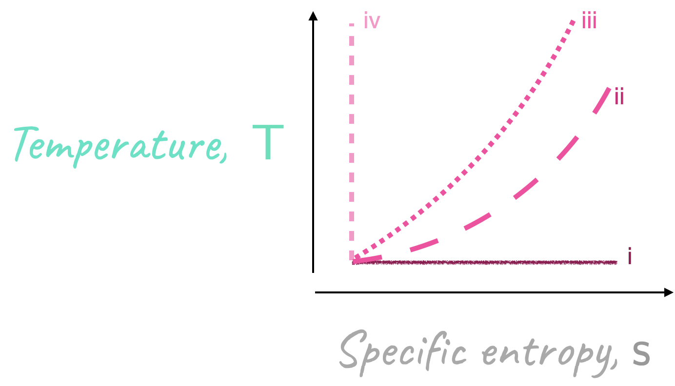
For a perfect gas, \(\require{color}{\color[rgb]{0.986252,0.007236,0.027423}h} = {\color[rgb]{0.986252,0.007236,0.027423}c}_{\color[rgb]{0.315209,0.728565,0.037706}p} {\color[rgb]{0.164799,0.878862,0.723179}T} + constant\). Hence, a constant \(\require{color}{\color[rgb]{0.986252,0.007236,0.027423}h}\) line is a constant \(\require{color}{\color[rgb]{0.164799,0.878862,0.723179}T}\) line.
We know that for a constant pressure process
\[ \large \require{color} {\color[rgb]{0.164799,0.878862,0.723179}T}{\color[rgb]{0.599997,0.600015,0.600005}ds} = {\color[rgb]{0.986252,0.007236,0.027423}dh} - {\color[rgb]{0.918231,0.469102,0.038229}\nu} {\color[rgb]{0.315209,0.728565,0.037706}dp} = {\color[rgb]{0.986252,0.007236,0.027423}dh} \]
So for a perfect gas
\[ \large \require{color} {\color[rgb]{0.986252,0.007236,0.027423}dh} = {\color[rgb]{0.986252,0.007236,0.027423}c}_{\color[rgb]{0.315209,0.728565,0.037706}p} {\color[rgb]{0.164799,0.878862,0.723179}dT} \Rightarrow \frac{{\color[rgb]{0.164799,0.878862,0.723179}dT}}{{\color[rgb]{0.599997,0.600015,0.600005}ds}} = \frac{{\color[rgb]{0.164799,0.878862,0.723179}T}}{{\color[rgb]{0.986252,0.007236,0.027423}c}_{\color[rgb]{0.315209,0.728565,0.037706}p}} \]
we anticipate a curve with a positive slope with the gradient increasing with temperature.
\[ \large \require{color} \mathsf{\frac{{\color[rgb]{0.164799,0.878862,0.723179}dT}}{{\color[rgb]{0.599997,0.600015,0.600005}ds}} = \frac{{\color[rgb]{0.164799,0.878862,0.723179}T}}{{\color[rgb]{0.878548,0.880173,0.060757}c}_{\color[rgb]{0.079785,0.618358,0.483717}V}} } \]
where \({\color[rgb]{0.986252,0.007236,0.027423}c}_{\color[rgb]{0.315209,0.728565,0.037706}p} > {\color[rgb]{0.878548,0.880173,0.060757}c}_{\color[rgb]{0.079785,0.618358,0.483717}V}\), and thus the trend for this is the same as in ii but with an increased gradient.