L9 examples

Problem 1

A two-dimensional air flow has circular streamlines, as shown in the figure.

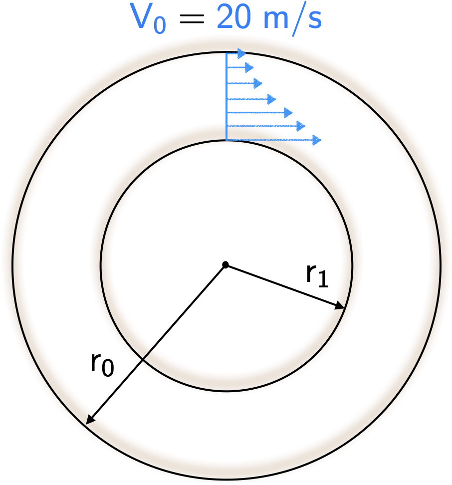
The velocity distribution is given by \(\require{color}{\color[rgb]{0.059472,0.501943,0.998465}V}\left(r\right) = c/r\), where \(\mathsf{c}\) is a constant and \(\mathsf{r}\) is the radial distance, i.e., the velocity is a function of the radius. At a radius of \(\mathsf{r}_{0} = 0.2 \; m\) the velocity is \(\require{color}\mathsf{{\color[rgb]{0.059472,0.501943,0.998465}V}_{0}=20 \; m/s}\). Assume the air is incompressible with a density \(\require{color}{\color[rgb]{0.918231,0.469102,0.038229}\rho } = {\color[rgb]{0.918231,0.469102,0.038229}1.2 \; kg/m^3}\).

• Calculate the pressure difference between the streamlines at \(\mathsf{r=r_{0}}\) and \(\mathsf{r=r_1=0.1 \; m}\).
• Prove whether or not Bernoulli’s equation can be applied between the streamlines at different radii.

Solution

Based on the problem description above, it is clear that

\[ \large \require{color}{\color[rgb]{0.059472,0.501943,0.998465}V}\left( r = r_0 \right) = \frac{c}{r_0} = {\color[rgb]{0.059472,0.501943,0.998465}V}_0 \Rightarrow c = {\color[rgb]{0.059472,0.501943,0.998465}V}_0 r_0 \]

From our study of streamlines, we know that the pressure gradient normal to a streamline with a radius of curvature is given by \(\require{color}d{\color[rgb]{0.315209,0.728565,0.037706}p} / dr = {\color[rgb]{0.918231,0.469102,0.038229}\rho}{\color[rgb]{0.059472,0.501943,0.998465}V}^2 / r\). Thus, we can write \[ \large \frac{d{\color[rgb]{0.315209,0.728565,0.037706}p}}{dr} = {\color[rgb]{0.918231,0.469102,0.038229}\rho} \frac{{\color[rgb]{0.059472,0.501943,0.998465}V}^2}{r} = {\color[rgb]{0.918231,0.469102,0.038229}\rho} \frac{\left( \frac{c}{r} \right)^2 }{r} = {\color[rgb]{0.918231,0.469102,0.038229}\rho} \frac{\left( \frac{{\color[rgb]{0.059472,0.501943,0.998465}V}_0 r_0}{r} \right)^2 }{r} \]

\[ \large \require{color}\Rightarrow d{\color[rgb]{0.315209,0.728565,0.037706}p} = {\color[rgb]{0.918231,0.469102,0.038229}\rho } \left( {\color[rgb]{0.059472,0.501943,0.998465}V}_{0} r_{0}\right)^2 \frac{dr}{r^3} \]

\[ \large \require{color}\Rightarrow \int_{0^{\ast}}^{1^{\ast}} d{\color[rgb]{0.315209,0.728565,0.037706}p} = {\color[rgb]{0.918231,0.469102,0.038229}\rho } {\color[rgb]{0.059472,0.501943,0.998465}V}_{0}^2 r_{0}^2 \cdot \int_{0^{\ast}}^{1^{\ast}} \frac{dr}{r^3} = {\color[rgb]{0.918231,0.469102,0.038229}\rho } {\color[rgb]{0.059472,0.501943,0.998465}V}_{0}^2 r_{0}^2 \cdot \left(- \frac{1}{2} \right) \left|\frac{1}{r^{2}}\right|_{r_{0}}^{r_{1}} \]

This yields

\[ \large \require{color}{\color[rgb]{0.315209,0.728565,0.037706}p}_{0} - {\color[rgb]{0.315209,0.728565,0.037706}p}_{1} = \frac{{\color[rgb]{0.918231,0.469102,0.038229}\rho } {\color[rgb]{0.059472,0.501943,0.998465}V}_{0}^2 r_{0}^2}{2} \left[ \frac{1}{r_{1}^2} - \frac{1}{r_{0}^2 }\right] = \frac{{\color[rgb]{0.918231,0.469102,0.038229}\rho } {\color[rgb]{0.059472,0.501943,0.998465}V}_{0}^2}{2} \left[ \left( \frac{r_{0}}{r_{1}}\right)^2 - 1\right] \]

Plugging in the values, we arrive at

\[ \large \require{color}= \frac{1.2 \times 20^2}{2}\left(2^2 - 1\right) = 720 \; Pa. \]

Bernoulli’s equation is applicable if the stagnation pressure (Bernoulli’s constant) across streamlines at different \(r\) values remains the same. In other words, we need to demonstrate that

\[ \large \require{color}\frac{d\left({\color[rgb]{0.315209,0.728565,0.037706}p} + \frac{1}{2}\rho {\color[rgb]{0.059472,0.501943,0.998465}V}^2\right)}{dr} \equiv 0 \; \; \textsf{for all r's.} \]

Now, since

\[ \large \require{color}\frac{d{\color[rgb]{0.315209,0.728565,0.037706}p}}{dr} = {\color[rgb]{0.918231,0.469102,0.038229}\rho } \frac{{\color[rgb]{0.059472,0.501943,0.998465}V}^2}{r} , \; \; \; and \; \; \; \frac{d\left(\frac{1}{2}{\color[rgb]{0.918231,0.469102,0.038229}\rho } {\color[rgb]{0.059472,0.501943,0.998465}V}^2 \right)}{dr} = \rho {\color[rgb]{0.059472,0.501943,0.998465}V} \frac{dV}{dr} = {\color[rgb]{0.918231,0.469102,0.038229}\rho } {\color[rgb]{0.059472,0.501943,0.998465}V} \underbrace{ {\color[rgb]{0.059472,0.501943,0.998465}V}_{0}r_{0}}_{c} \frac{d\left(r^{-1}\right)}{dr} = -\frac{{\color[rgb]{0.918231,0.469102,0.038229}\rho } {\color[rgb]{0.059472,0.501943,0.998465}V}^2}{r} \]

we have

\[ \large \require{color}\frac{d \left({\color[rgb]{0.315209,0.728565,0.037706}p} + \frac{1}{2} \rho {\color[rgb]{0.059472,0.501943,0.998465}V}^2 \right)}{dr} = {\color[rgb]{0.918231,0.469102,0.038229}\rho } \frac{{\color[rgb]{0.059472,0.501943,0.998465}V}^2}{r} - {\color[rgb]{0.918231,0.469102,0.038229}\rho}\frac{{\color[rgb]{0.059472,0.501943,0.998465}V}^2}{r} \equiv 0. \]

This completes our proof. Thus, stagnation pressure across streamlines does not change and the expression is applicable to the whole flow field.