L5 examples

Problem 1

What is the velocity of the air if a Pitot static tube measures \(\require{color}{\color[rgb]{0.315209,0.728565,0.037706}p_1} = {\color[rgb]{0.315209,0.728565,0.037706}101,325 \; N/m^2}\) and \(\require{color}{\color[rgb]{0.315209,0.728565,0.037706}p_2} = {\color[rgb]{0.315209,0.728565,0.037706}95,000 \; N/m^2}\). Assume the density of air is \(\require{color}{\color[rgb]{0.918231,0.469102,0.038229}\rho } = {\color[rgb]{0.918231,0.469102,0.038229}1.25 \; kg/m^3}\).

Aircraft	Pitot static tube

Solution

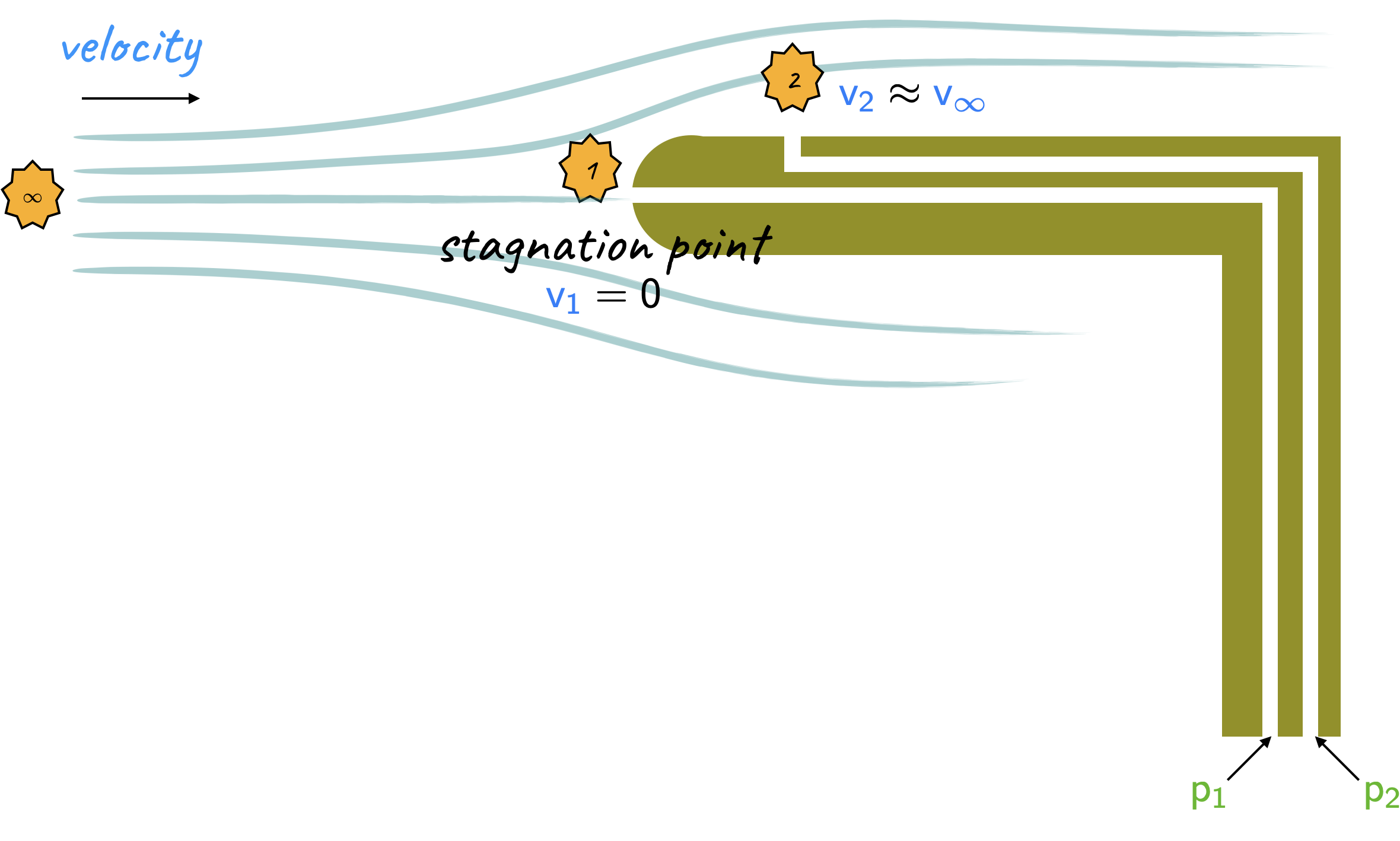Consider the streamline from \(\infty\) to station \(1\).

\[ \large \require{color}{\color[rgb]{0.315209,0.728565,0.037706}p_{\infty}} + \frac{1}{2} {\color[rgb]{0.918231,0.469102,0.038229}\rho }{\color[rgb]{0.059472,0.501943,0.998465}v_{\infty}}^2 = {\color[rgb]{0.315209,0.728565,0.037706}p_1 }+ \frac{1}{2}{\color[rgb]{0.918231,0.469102,0.038229}\rho} {\color[rgb]{0.059472,0.501943,0.998465}v_1}^2 = {\color[rgb]{0.315209,0.728565,0.037706}p_1} \]

\[ \large \require{color}\Rightarrow {\color[rgb]{0.315209,0.728565,0.037706}p_1} = {\color[rgb]{0.315209,0.728565,0.037706}p_{\infty}} + \frac{1}{2} {\color[rgb]{0.918231,0.469102,0.038229}\rho }{\color[rgb]{0.059472,0.501943,0.998465}v_{\infty}}^2 \]

as \(\require{color}{\color[rgb]{0.059472,0.501943,0.998465}v_1} = 0\). Now consider the flow from \(\infty\) to station \(2\), i.e.,

\[ \large \require{color}{\color[rgb]{0.315209,0.728565,0.037706}p_{\infty} }+ \frac{1}{2}{\color[rgb]{0.918231,0.469102,0.038229} \rho} {\color[rgb]{0.059472,0.501943,0.998465}v_{\infty}}^2 = {\color[rgb]{0.315209,0.728565,0.037706}p_2 }+ \frac{1}{2} {\color[rgb]{0.918231,0.469102,0.038229}\rho} {\color[rgb]{0.059472,0.501943,0.998465}v_{2}}^2. \]

However, as \(\require{color}{\color[rgb]{0.059472,0.501943,0.998465}v_2} = {\color[rgb]{0.059472,0.501943,0.998465}v_{\infty}}\), this implies \(\require{color}{\color[rgb]{0.315209,0.728565,0.037706}p_2} = {\color[rgb]{0.315209,0.728565,0.037706}p_{\infty}}\).

Thus, from these equations we have

\[ \large \require{color}{\color[rgb]{0.315209,0.728565,0.037706}p_1} - {\color[rgb]{0.315209,0.728565,0.037706}p_2 }= \frac{1}{2} {\color[rgb]{0.918231,0.469102,0.038229}\rho} {\color[rgb]{0.059472,0.501943,0.998465}v_{\infty}}^2 \Rightarrow {\color[rgb]{0.059472,0.501943,0.998465}v_{\infty} }= \sqrt{\frac{2 \left({\color[rgb]{0.315209,0.728565,0.037706}p_1} - {\color[rgb]{0.315209,0.728565,0.037706}p_2} \right) }{{\color[rgb]{0.918231,0.469102,0.038229}\rho}}} \]

Plugging in the provided values yields:

Code

import numpy as np

p_1 = 101325
p_2 = 95000
rho = 1.25
v_inf = np.sqrt(2 * (p_1 - p_2) / rho)
print(str(v_inf)+' m/s')

100.59821071967433 m/s

Problem 2

What is the drag that acts on the previously encountered (see Lecture 3 slides) half-body in a channel if \(\require{color}{\color[rgb]{0.918231,0.469102,0.038229}\rho } = {\color[rgb]{0.918231,0.469102,0.038229}1.25 \; kg/m^3}\), \(H= 10\; m\), \(\require{color}{\color[rgb]{0.064095,0.501831,0.501977}h}={\color[rgb]{0.064095,0.501831,0.501977}1 \; m}\), \(w=2 \; m\), and \(\require{color}{\color[rgb]{0.059472,0.501943,0.998465}v_1 } = {\color[rgb]{0.059472,0.501943,0.998465}20 \; m/s }\).

channel

Solution

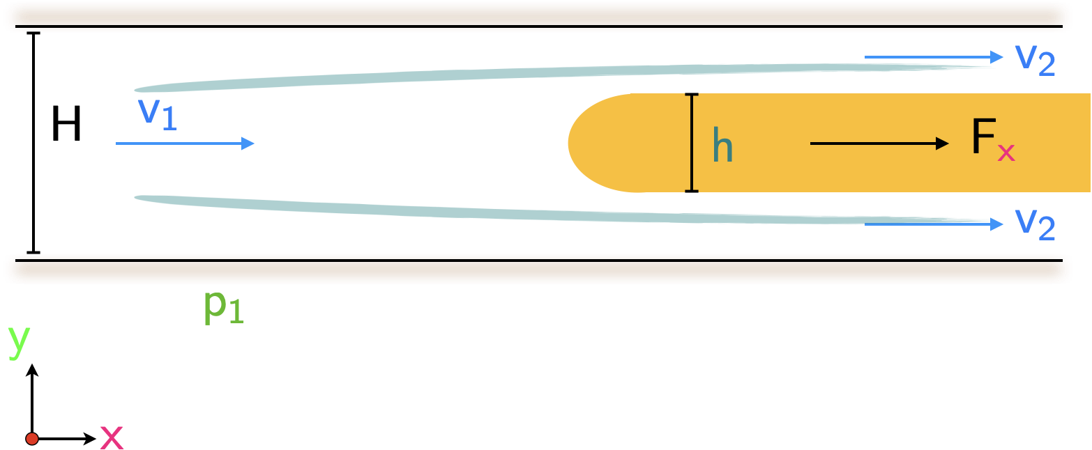
In Lecture 3, we had observed that the mass flux through the control volume is given by

\[ \large \require{color}\dot{m} = {\color[rgb]{0.918231,0.469102,0.038229}\rho} {\color[rgb]{0.059472,0.501943,0.998465}v_1} H w \]

where \(w\) is the width into the page of the channel. Recall from before, we had utilized continuity within the control volume to arrive at

\[ \large \require{color}{\color[rgb]{0.059472,0.501943,0.998465}v_2} = {\color[rgb]{0.059472,0.501943,0.998465}v_1} \frac{H}{H - {\color[rgb]{0.064095,0.501831,0.501977}h}}. \]

Now, we can use the steady flow momentum equation along the horizontal direction to yield an expression for the force \(\require{color}F_{{\color[rgb]{0.986048,0.008333,0.501924}x}}\). Let us break this up into the mass fluxes and the pressure forces.

\[ \large \require{color}\sum \dot{m} {\color[rgb]{0.059472,0.501943,0.998465}v }= \dot{m}_{out} {\color[rgb]{0.059472,0.501943,0.998465}v_{out}} - \dot{m}_{in} {\color[rgb]{0.059472,0.501943,0.998465}v_{in}} = \dot{m}_{in} \left({\color[rgb]{0.059472,0.501943,0.998465} v_{out}} - {\color[rgb]{0.059472,0.501943,0.998465}v_{in}} \right) \]

\[ \large \require{color}= \underbrace{{\color[rgb]{0.990448,0.502245,0.032881}\rho} {\color[rgb]{0.059472,0.501943,0.998465}v_1} H w}_{\dot{m}_{in}} \left( {\color[rgb]{0.059472,0.501943,0.998465}v_1} \frac{H}{H-{\color[rgb]{0.064095,0.501831,0.501977}h}} - {\color[rgb]{0.059472,0.501943,0.998465}v_{1}} \right) = {\color[rgb]{0.918231,0.469102,0.038229}\rho} w {\color[rgb]{0.059472,0.501943,0.998465}v_{1}}^2 \frac{H{\color[rgb]{0.064095,0.501831,0.501977}h}}{H-{\color[rgb]{0.064095,0.501831,0.501977}h}} \]

Now, to work out the force acting along the right-hand control surface, we need to isolate the front part of the half-body from the remaining part. It is possible to side-step this issue by placing an imaginary cut through the half-body, and permitting the gap to be filled with the same fluid at pressure \(\require{color}{\color[rgb]{0.315209,0.728565,0.037706}p_2}\). This yields the diagram below:

channel

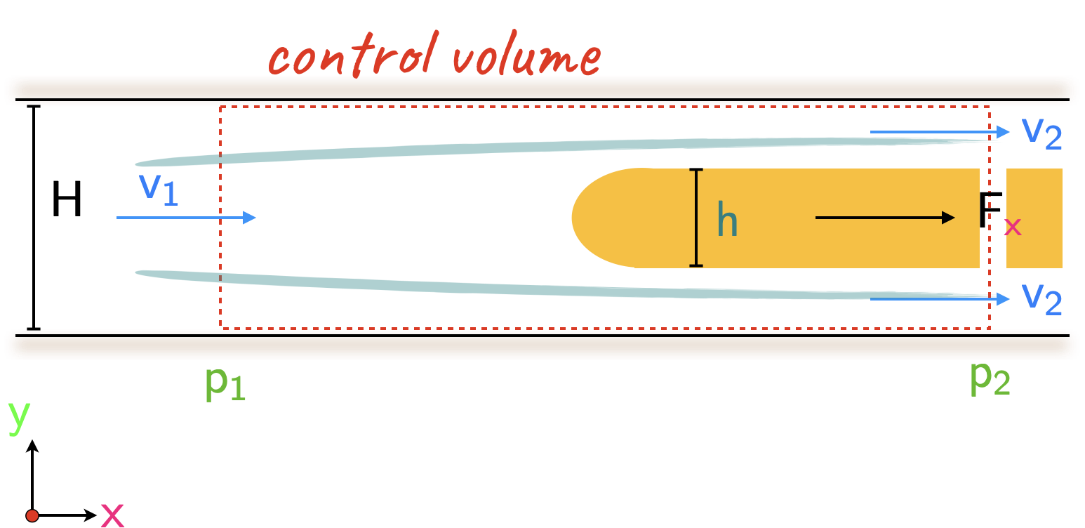
The total pressure force acting on the fluid along the \({\color[rgb]{0.986048,0.008333,0.501924}x-}\)direction is given by

\[ \large \require{color}\sum {\color[rgb]{0.315209,0.728565,0.037706}p} A = {\color[rgb]{0.315209,0.728565,0.037706}p_1} H w - {\color[rgb]{0.315209,0.728565,0.037706}p_2 }H w \]

Recognizing that the force \(F_{{\color[rgb]{0.986048,0.008333,0.501924}x}}\) is equal and opposite to the drag, \(D\), experienced by the body, we have

\[ \large \require{color}F_{{\color[rgb]{0.986048,0.008333,0.501924}x}} = -D = {\color[rgb]{0.990448,0.502245,0.032881}\rho} w {\color[rgb]{0.059472,0.501943,0.998465}v_1}^2 \frac{Hh}{H-{\color[rgb]{0.064095,0.501831,0.501977}h}} - \left({\color[rgb]{0.315209,0.728565,0.037706}p_1} - {\color[rgb]{0.315209,0.728565,0.037706}p_2} \right) H w. \]

Next, we need to determine the relationship between pressures \(\require{color}{\color[rgb]{0.315209,0.728565,0.037706}p_1}\) and \(\require{color}{\color[rgb]{0.315209,0.728565,0.037706}p_2}\). At the entry and exit to the control volume, we assume the streamlines are parallel and that the pressure is uniform throughout—not varying with depth. Applying Bernoulli’s principle between stations \(1\) and \(2\) yields

\[ \large \require{color}{\color[rgb]{0.315209,0.728565,0.037706}p_1} + \frac{1}{2} {\color[rgb]{0.918231,0.469102,0.038229}\rho }{\color[rgb]{0.059472,0.501943,0.998465}v_1}^2 = {\color[rgb]{0.315209,0.728565,0.037706}p_2} + \frac{1}{2} {\color[rgb]{0.918231,0.469102,0.038229}\rho} {\color[rgb]{0.059472,0.501943,0.998465}v_{2}}^2. \]

Using the expression for \(\require{color}{\color[rgb]{0.059472,0.501943,0.998465}v_2}\) in terms of \(\require{color}{\color[rgb]{0.059472,0.501943,0.998465}v_1}\) yields

\[ \large \require{color}{\color[rgb]{0.315209,0.728565,0.037706}p_1} - {\color[rgb]{0.315209,0.728565,0.037706}p_2} = \frac{{\color[rgb]{0.918231,0.469102,0.038229}\rho}}{2} {\color[rgb]{0.059472,0.501943,0.998465}v_1}^2 \left( \frac{H^2}{\left(H - {\color[rgb]{0.064095,0.501831,0.501977}h} \right)^2 } - 1 \right) \]

\[ \large \require{color}=\frac{{\color[rgb]{0.918231,0.469102,0.038229}\rho}}{2} {\color[rgb]{0.059472,0.501943,0.998465}v_1}^2 {\color[rgb]{0.064095,0.501831,0.501977}h} \frac{2H - {\color[rgb]{0.064095,0.501831,0.501977}h}}{\left( H - {\color[rgb]{0.064095,0.501831,0.501977}h} \right)^2 } \]

Thus, for the force we obtain

\[ \large \require{color}F_{{\color[rgb]{0.986048,0.008333,0.501924}x}} = {\color[rgb]{0.990448,0.502245,0.032881}\rho} w {\color[rgb]{0.059472,0.501943,0.998465}v_1}^2 \frac{H{\color[rgb]{0.064095,0.501831,0.501977}h}}{H-{\color[rgb]{0.064095,0.501831,0.501977}h}} - \frac{1}{2}{\color[rgb]{0.918231,0.469102,0.038229} \rho} {\color[rgb]{0.059472,0.501943,0.998465}v_1}^2 {\color[rgb]{0.064095,0.501831,0.501977}h} \frac{2H - {\color[rgb]{0.064095,0.501831,0.501977}h}}{\left(H - {\color[rgb]{0.064095,0.501831,0.501977}h}\right)^2}Hw \]

\[ \large \require{color}= \frac{w {\color[rgb]{0.918231,0.469102,0.038229}\rho} {\color[rgb]{0.059472,0.501943,0.998465}v_1}^2}{2} \left[ 2 \frac{H{\color[rgb]{0.064095,0.501831,0.501977}h}}{H - {\color[rgb]{0.064095,0.501831,0.501977}h}} - H{\color[rgb]{0.064095,0.501831,0.501977}h} \frac{2H - {\color[rgb]{0.064095,0.501831,0.501977}h}}{\left(H -{\color[rgb]{0.064095,0.501831,0.501977} h} \right)^2 } \right] \]

\[ \large \require{color}= \frac{w {\color[rgb]{0.918231,0.469102,0.038229}\rho} {\color[rgb]{0.059472,0.501943,0.998465}v_1}^2}{2} \left[ \frac{2H{\color[rgb]{0.064095,0.501831,0.501977}h} \left(H - {\color[rgb]{0.064095,0.501831,0.501977}h} \right) - H{\color[rgb]{0.064095,0.501831,0.501977}h} \left(2 H - {\color[rgb]{0.064095,0.501831,0.501977}h} \right) }{\left(H - {\color[rgb]{0.064095,0.501831,0.501977}h} \right)^2} \right] \]

\[ \large \require{color}= \frac{w {\color[rgb]{0.918231,0.469102,0.038229}\rho} {\color[rgb]{0.059472,0.501943,0.998465}v_1}^2}{2} \left[ \frac{-H{\color[rgb]{0.064095,0.501831,0.501977}h}^2}{\left(H - {\color[rgb]{0.064095,0.501831,0.501977}h} \right)^2} \right] \]

As a side, note that for very large \(\require{color}H >> {\color[rgb]{0.064095,0.501831,0.501977}h}\), the drag force fanishes. Now that we have the expression above, we can plug in the provided numerical values.

Code

H = 10 
h = 1
v_1 = 20
rho = 1.25
w = 2
F_x = w * 0.5 * rho * v_1**2 * (-(H * h**2) / (H - h)**2)
print(str(F_x)+' N')

-61.72839506172839 N