L18 examples
Problem 1
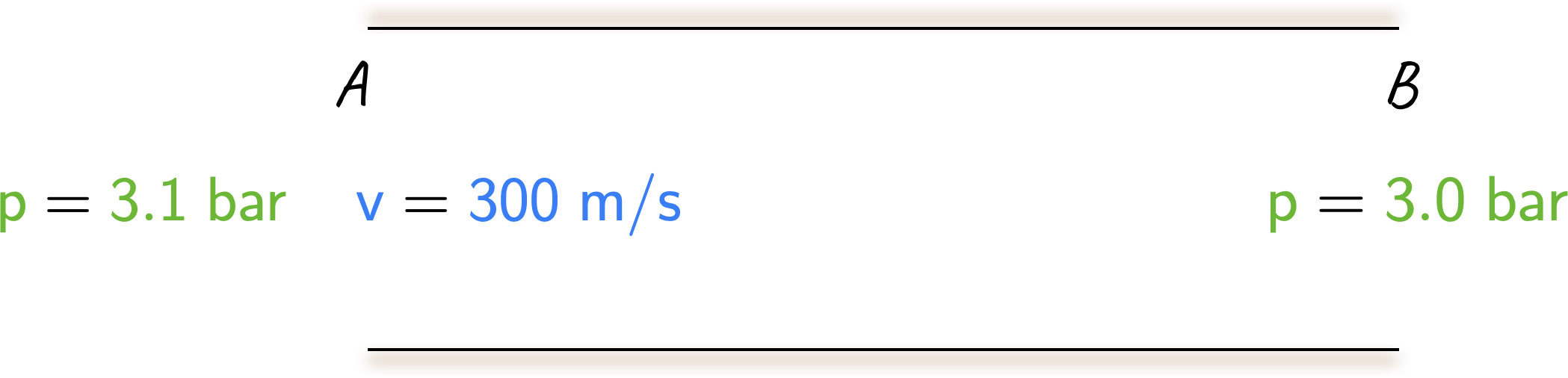
Air flows in a pipe with a high velocity at which friction forces are significant. Heat transfer occurs through the pipe wall such that the air temperature inside remains constant at \(\require{color}{\color[rgb]{0.164799,0.878862,0.723179}305\; K}\). At point A in the pipe the velocity is \(\require{color}{\color[rgb]{0.059472,0.501943,0.998465}300\; m/s}\) and the pressure is \(\require{color}{\color[rgb]{0.315209,0.728565,0.037706}3.1 \; bar}\). At point B the pressure is \(\require{color}{\color[rgb]{0.315209,0.728565,0.037706}3.0 \; bar}\). Is B upstream or downstream of A?
Solution
We can apply the equation
\[ \large \require{color}{\color[rgb]{0.599997,0.600015,0.600005}s_e} - {\color[rgb]{0.599997,0.600015,0.600005}s_i} = \sum \frac{{\color[rgb]{0.334690,0.296180,0.998454}q_i}}{{\color[rgb]{0.164799,0.878862,0.723179}T_i}} + {\color[rgb]{0.599997,0.600015,0.600005}\Delta s}_{irrev} \]
to work out \(\require{color}{\color[rgb]{0.599997,0.600015,0.600005}\Delta s}_{irrev}\) assuming the flow is from A to B due to the pressure difference. If it turns out that \(\require{color}{\color[rgb]{0.599997,0.600015,0.600005}\Delta s}_{irrev}\) is less than zero, then we know this assumption cannot be true, as the irreversibilities must result in a positive entropy contribution.
To begin, consider that
\[ \large \require{color} \dot{m} = {\color[rgb]{0.918231,0.469102,0.038229}\rho_A} {\color[rgb]{0.059472,0.501943,0.998465}v_A} A = {\color[rgb]{0.918231,0.469102,0.038229}\rho_B} {\color[rgb]{0.059472,0.501943,0.998465}v_B} A \Rightarrow \frac{{\color[rgb]{0.315209,0.728565,0.037706}p_A}}{R {\color[rgb]{0.164799,0.878862,0.723179}T}} {\color[rgb]{0.059472,0.501943,0.998465}v_A} = \frac{{\color[rgb]{0.315209,0.728565,0.037706}p_B}}{R {\color[rgb]{0.164799,0.878862,0.723179}T}} {\color[rgb]{0.059472,0.501943,0.998465}v_B} \Rightarrow {\color[rgb]{0.059472,0.501943,0.998465}v_{B}} = {\color[rgb]{0.059472,0.501943,0.998465}v_A} \frac{{\color[rgb]{0.315209,0.728565,0.037706}p_A}}{{\color[rgb]{0.315209,0.728565,0.037706}p_B}} \]
This leads to
\[ \large \require{color} {\color[rgb]{0.059472,0.501943,0.998465}v_{B}} = \frac{{\color[rgb]{0.315209,0.728565,0.037706}3.1}}{{\color[rgb]{0.315209,0.728565,0.037706}3.0}} \times {\color[rgb]{0.059472,0.501943,0.998465}300} = {\color[rgb]{0.059472,0.501943,0.998465}310 \; m/s} \]
Assuming the flow goes from A to B we can apply the SFEE to arrive at
\[ \large \require{color} {\color[rgb]{0.334690,0.296180,0.998454}q} - {\color[rgb]{0.562040,0.190215,0.568721}w_{x}} = \left({\color[rgb]{0.986252,0.007236,0.027423}h_B} + \frac{1}{2} {\color[rgb]{0.059472,0.501943,0.998465}v_B}^2 + g {\color[rgb]{0.986047,0.008333,0.501923}z_{B}} \right) - \left( {\color[rgb]{0.986252,0.007236,0.027423}h_A} + \frac{1}{2} {\color[rgb]{0.059472,0.501943,0.998465}v_A}^2 + g {\color[rgb]{0.986047,0.008333,0.501923}z_{A}} \right) \; \; \; \; \; {\color[rgb]{0.986252,0.007236,0.027423}\Delta h} = {\color[rgb]{0.986252,0.007236,0.027423}c}_{{\color[rgb]{0.315209,0.728565,0.037706}p}} {\color[rgb]{0.164799,0.878862,0.723179}\Delta T} = 0. \]
Setting \(\require{color}{\color[rgb]{0.562040,0.190215,0.568721}w_{x}} = 0\) and ignoring the potential energy terms, we have
\[ \large \require{color} q = \frac{1}{2} \left( {\color[rgb]{0.059472,0.501943,0.998465}v_B}^2 - {\color[rgb]{0.059472,0.501943,0.998465}v_A}^2 \right) = \frac{1}{2} \left( {\color[rgb]{0.059472,0.501943,0.998465}310}^2 - {\color[rgb]{0.059472,0.501943,0.998465}300}^2 \right) = {\color[rgb]{0.334690,0.296180,0.998454}3050 \frac{J}{kg}} \]
We can also work out the entropy, i.e.,
\[ \large \require{color} {\color[rgb]{0.599997,0.600015,0.600005}s_{B}} - {\color[rgb]{0.599997,0.600015,0.600005}s_{A}} = {\color[rgb]{0.986252,0.007236,0.027423}c}_{\color[rgb]{0.315209,0.728565,0.037706}p} \; ln \left( \frac{{\color[rgb]{0.059472,0.501943,0.998465}T_B}}{{\color[rgb]{0.059472,0.501943,0.998465}T_A}} \right) - R \; ln \left( \frac{{\color[rgb]{0.315209,0.728565,0.037706}p_B}}{{\color[rgb]{0.315209,0.728565,0.037706}p_A}} \right) \]
where we recognize that the first term on the right-hand side must be zero because the system is isothermal. This leads to
\[ \large \require{color} {\color[rgb]{0.599997,0.600015,0.600005}s_{B}} - {\color[rgb]{0.599997,0.600015,0.600005}s_{A}} = - R ln \left( \frac{{\color[rgb]{0.315209,0.728565,0.037706}p_B}}{{\color[rgb]{0.315209,0.728565,0.037706}p_A}} \right) = R \; ln \left(\frac{{\color[rgb]{0.315209,0.728565,0.037706}p_A}}{{\color[rgb]{0.315209,0.728565,0.037706}p_B}} \right) = 287 \times ln \left( \frac{{\color[rgb]{0.315209,0.728565,0.037706}3.1}}{{\color[rgb]{0.315209,0.728565,0.037706}3}} \right) = {\color[rgb]{0.599997,0.600015,0.600005}9.41 \; \frac{J}{kg \cdot K}} \]
Note that
\[ \large \require{color} {\color[rgb]{0.599997,0.600015,0.600005}\Delta s_{irrev}} = \left({\color[rgb]{0.599997,0.600015,0.600005}s_B} - {\color[rgb]{0.599997,0.600015,0.600005}s_A} \right) - \frac{{\color[rgb]{0.334690,0.296180,0.998454}q}}{{\color[rgb]{0.164799,0.878862,0.723179}T}} \]
because at constant temperature \(\require{color}\sum \frac{{\color[rgb]{0.334690,0.296180,0.998454}q_j}}{{\color[rgb]{0.164799,0.878862,0.723179}T_j}} = \frac{{\color[rgb]{0.334690,0.296180,0.998454}q}}{{\color[rgb]{0.164799,0.878862,0.723179}T}}\). Thus
\[ \large \require{color} {\color[rgb]{0.599997,0.600015,0.600005}\Delta s_{irrev}} = {\color[rgb]{0.599997,0.600015,0.600005}9.41 \; \frac{J}{kg \cdot K}} - \frac{{\color[rgb]{0.334690,0.296180,0.998454}3050}}{{\color[rgb]{0.164799,0.878862,0.723179}305}} = {\color[rgb]{0.599997,0.600015,0.600005}-0.59 \; \frac{J}{kg \cdot K}} \]
This is impossible and thus our original assumption must be wrong. Therefore, the flow must be from B to A.
Note: This rather unusual behavior of flow moving against the pressure gradient arises because the velocity is close to the speed of sound (as we will see in the compressible flow section of this course). At this speed it is unlikely that heat transfer could be fast enough to maintain isothermal flow. This problem could also have been solved using the SFME to work out the frictional force which must oppose the flow.
Problem 2
A pump discharges 600 liters of water per minute. The inlet and delivery pipes are of the same diameter and at the same level. The pressure at the inlet is \(\require{color}{\color[rgb]{0.315209,0.728565,0.037706}1.0 \; bar}\), and that at the exit is \(\require{color}{\color[rgb]{0.315209,0.728565,0.037706}100.0 \; bar}\). Calculate the minimum shaft power required to drive the pump.
Solution
The flow is incompressible, i.e., \(\require{color}{\color[rgb]{0.918231,0.469102,0.038229}\nu} = 1 / {\color[rgb]{0.918231,0.469102,0.038229}\rho} = constant\), so the expression for shaft work can be integrated:
\[ \large \require{color} -{\color[rgb]{0.562040,0.190215,0.568721}w_{x}} = \int_{i}^{e} {\color[rgb]{0.918231,0.469102,0.038229}\nu} {\color[rgb]{0.315209,0.728565,0.037706}dp} + \left( \frac{1}{2} {\color[rgb]{0.059472,0.501943,0.998465}v_{e}}^2 + g{\color[rgb]{0.986047,0.008333,0.501923}z_{e}} \right) - \left( \frac{1}{2} {\color[rgb]{0.059472,0.501943,0.998465}v_i}^2 + g{\color[rgb]{0.986047,0.008333,0.501923}z_i} \right) \]
\[ \large \require{color} -{\color[rgb]{0.562040,0.190215,0.568721}w_{x}} = \frac{\left( {\color[rgb]{0.315209,0.728565,0.037706}p_e} - {\color[rgb]{0.315209,0.728565,0.037706}p_i} \right)}{\rho} + \left( \frac{1}{2} {\color[rgb]{0.059472,0.501943,0.998465}v_e}^2 + g{\color[rgb]{0.986047,0.008333,0.501923}z_{e}} \right) - \left( \frac{1}{2} {\color[rgb]{0.059472,0.501943,0.998465}v_i}^2 + g{\color[rgb]{0.986047,0.008333,0.501923}z_{i}}\right) \]
Since the inlet and exit have the same diameter and density is constant, the velocities are the same and there is no change in the kinetic energy. Additionally, as the inlet and exit are on the same level, there is no reason why the potential energy should change. Thus, the specific shaft work is given by:
\[ \large \require{color} -{\color[rgb]{0.562040,0.190215,0.568721}w_{x}} = \frac{\left( {\color[rgb]{0.315209,0.728565,0.037706}p_e} - {\color[rgb]{0.315209,0.728565,0.037706}p_i} \right)}{{\color[rgb]{0.918231,0.469102,0.038229}\rho}}. \]
The shaft power is obtained by multiplying the specific shaft work by the massflow rate, i.e.,
\[ \large \require{color} -{\color[rgb]{0.562040,0.190215,0.568721}W_{x}} = \dot{m} \times -{\color[rgb]{0.562040,0.190215,0.568721}w_{x}} = \frac{\rho \mathcal{Q} \left({\color[rgb]{0.315209,0.728565,0.037706}p_e} - {\color[rgb]{0.315209,0.728565,0.037706}p_i} \right) }{{\color[rgb]{0.918231,0.469102,0.038229}\rho}} = \mathcal{Q} {\color[rgb]{0.315209,0.728565,0.037706}\Delta p } \]
where \(\mathcal{Q}\) is the volumetric flow rate. From the above, the minimum shaft power is
\[ \large \require{color} = \frac{600 \times 10^{-3} \; kg / minute}{60 \; sec / minute} \times \left( {\color[rgb]{0.315209,0.728565,0.037706}100 \times 10^5} - {\color[rgb]{0.315209,0.728565,0.037706}1 \times 10^5 }\right) = {\color[rgb]{0.562040,0.190215,0.568721}99 \; kW}. \]
Notes: This is the minimum work input because the flow has been assumed reversible. Also note that if the shaft work is set to zero, this yields teh familiar Bernoulli’s equation for incompressible, steady and inviscid (and thus reversible) flow.