Vector fields

Code

import numpy as np
import matplotlib.pyplot as plt
from matplotlib.cm import ScalarMappable

Overview

This notebook tries to describe various concepts pertaining to velocity (vector) fields. For ease in illustration, we will restrict our attention to velocity fields in 2D. To begin, consider the following velocity field:

\[ \large \require{color}{\color[rgb]{0.059472,0.501943,0.998465}v}_{\color[rgb]{0.986048,0.008333,0.501924}x} = 5 cos(3{\color[rgb]{0.986048,0.008333,0.501924}x}) + 3 {\color[rgb]{0.131302,0.999697,0.023594}y}^2 \]

\[ \large \require{color}{\color[rgb]{0.059472,0.501943,0.998465}v}_{\color[rgb]{0.131302,0.999697,0.023594}y} = 2 sin(4{\color[rgb]{0.131302,0.999697,0.023594}y}) - \left({\color[rgb]{0.986048,0.008333,0.501924}x} - 0.5 \right)^2 \]

From which we can work out the partial derivatives of velocity rather easily.

Code

x = np.linspace(-1, 1, 40)
y = np.linspace(-1, 1, 40)
X, Y = np.meshgrid(x, y)
vel_X = 5 * np.cos(3*X) + 3 * Y**2
vel_Y = 2 * np.sin(4*Y) - (X-0.5)**2

dvel_dX = -15 * np.sin(3*X) + 6 * Y
dvel_dY = 8 * np.cos(4*Y) - 2*(X-0.5)

Code

fig = plt.figure(figsize=(8,4))
c = plt.contourf(X, Y, vel_X, 30)
plt.colorbar(c)
plt.title(r'$v_x$')
plt.xlabel('x')
plt.ylabel('y')
plt.show()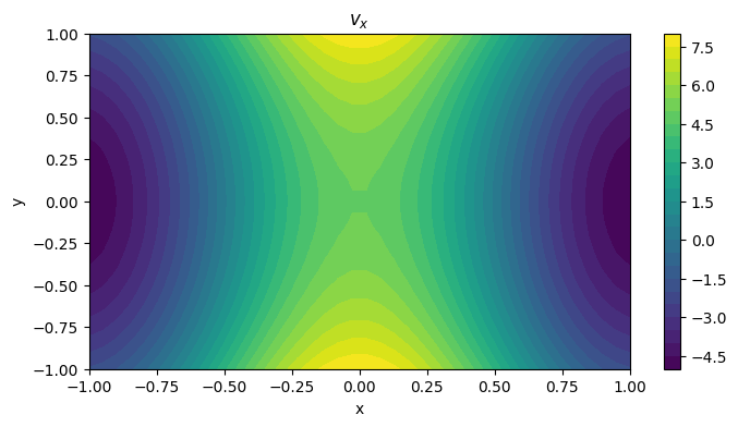

Code

fig = plt.figure(figsize=(8,4))
c = plt.contourf(X, Y, vel_Y, 30)
plt.colorbar(c)
plt.title(r'$v_y$')
plt.xlabel('x')
plt.ylabel('y')
plt.show()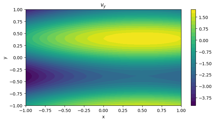

Once again, following from lecture, note how the two velocity components can have very different (independent) velocity variations across space. It will be useful to plot the velocity vectors over contours of the velocity magnitude.

Code

vel_mag = np.sqrt(vel_X**2 + vel_Y**2)

fig = plt.figure(figsize=(8,4))
c = plt.contourf(X, Y, vel_mag, 30)
plt.quiver(X, Y, vel_X, vel_Y, color='w')
plt.colorbar(c)
plt.title(r'Velocity, $\mathbf{v}$')
plt.xlabel('x')
plt.ylabel('y')
plt.show()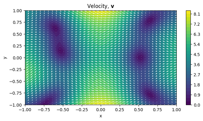

Divergence

To work out the location of the sources and sinks, we need to compute the divergence of this velocity field. Recall, the formula for the divergence:

\[ \large \require{color} \nabla \cdot \boldsymbol{{\color[rgb]{0.059472,0.501943,0.998465}v}} = \left(\left[\begin{array}{c} \partial/\partial {\color[rgb]{0.986048,0.008333,0.501924}x}\\ \partial/\partial {\color[rgb]{0.131302,0.999697,0.023594}y} \end{array}\right]\cdot\left[\begin{array}{c} {{\color[rgb]{0.059472,0.501943,0.998465}v}}_{{\color[rgb]{0.986048,0.008333,0.501924}x}}\\ {\color[rgb]{0.059472,0.501943,0.998465}v}_{{\color[rgb]{0.131302,0.999697,0.023594}y}} \end{array}\right]\right) \]

The tiny block of code below calculates the divergence in div. It also creates a new variable div_bool which is a matrix of divergence values. When the divergence is negative, all values are assigned -1. When the divergence is positive, all values are assigned 1, and when the divergence is close to zero, all values are assigned 0.

Code

div = dvel_dX + dvel_dY
div_bool = np.ones((div.shape[0], div.shape[1]))
for i in range(0, div.shape[0]):
    for j in range(0, div.shape[1]):
        if np.abs(div[i,j] - 0) < 0.01:
            div_bool[i,j] = 0.
        elif div[i,j] > 0:
            div_bool[i,j] = 1
        else:
            div_bool[i,j] = -1

The contour plot below plots div_bool.

Code

fig = plt.figure(figsize=(8,4))
vmin = -1
vmax = 1
c = plt.contourf(X, Y, div_bool, 80, vmin=vmin, vmax=vmax, cmap=plt.cm.gray)
cbar = fig.colorbar(
   ScalarMappable(norm=c.norm, cmap=c.cmap),
   ticks=[-1, 0, 1]
)
cbar.set_ticklabels(['Sink', 'Neutral', 'Source'])
plt.quiver(X, Y, vel_X, vel_Y, color='y')
plt.title(r'Divergence, $\nabla \cdot \mathbf{v}$')
plt.xlabel('x')
plt.ylabel('y')
plt.show()

/var/folders/34/0177579s72zfk8k1ytk34_9c0346k7/T/ipykernel_42334/1478740457.py:5: MatplotlibDeprecationWarning: Unable to determine Axes to steal space for Colorbar. Using gca(), but will raise in the future. Either provide the *cax* argument to use as the Axes for the Colorbar, provide the *ax* argument to steal space from it, or add *mappable* to an Axes.
  cbar = fig.colorbar(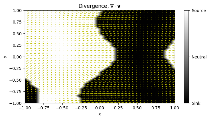

What the above plot shows is that the divergence is of velocity over a field provides a measure to delineate on average where the bulk of the flow is headed.

Advection

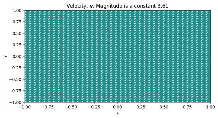
The advection operator was introduced in lecture as providing the variation of a quantity following the velocity. Consider a distinct velocity field given by

\[ \large \require{color}{\color[rgb]{0.059472,0.501943,0.998465}v}_{\color[rgb]{0.986048,0.008333,0.501924}x} = 3 \]

\[ \large \require{color}{\color[rgb]{0.059472,0.501943,0.998465}v}_{\color[rgb]{0.131302,0.999697,0.023594}y} = 2 \]

and a height field given by

\[ \large \require{color}h\left({\color[rgb]{0.986048,0.008333,0.501924}x}, {\color[rgb]{0.131302,0.999697,0.023594}y} \right) = -0.2 {\color[rgb]{0.131302,0.999697,0.023594}y}^2 - 0.2 {\color[rgb]{0.986048,0.008333,0.501924}x}^2 + 10 \]

Code

vel_X = 3 + 0 * X
vel_Y = 2 + 0 * Y
h =  -0.2*Y**2 - 0.2 * X**2 + 10

Code

fig = plt.figure(figsize=(8,4))
c = plt.contourf(X, Y, h, 30, cmap=plt.cm.jet)
plt.colorbar(c)
plt.title(r'$h$')
plt.xlabel('x')
plt.ylabel('y')
plt.show()

vel_mag = np.sqrt(vel_X**2 + vel_Y**2)

fig = plt.figure(figsize=(8,4))
c = plt.contourf(X, Y, vel_mag, 30)
plt.quiver(X, Y, vel_X, vel_Y, color='w')
plt.title(r'Velocity, $\mathbf{v}$. Magnitude is a constant '+str(np.around(vel_mag[0,0], 2)) )
plt.xlabel('x')
plt.ylabel('y')
plt.show()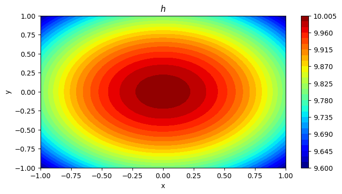

We now plot the output of the advection operator, which for a scalar field is given by

Code

dh_dX =  -2 * 0.2 * X
dh_dY = -2 * 0.2 * Y
advection_h = vel_X * dh_dX + vel_Y * dh_dY

fig = plt.figure(figsize=(8,4))
c = plt.contourf(X, Y,advection_h, 30, cmap=plt.cm.jet)
plt.colorbar(c)
plt.title(r'Advection operator $(\mathbf{v} \cdot \nabla ) h$')
plt.xlabel('x')
plt.ylabel('y')
plt.show()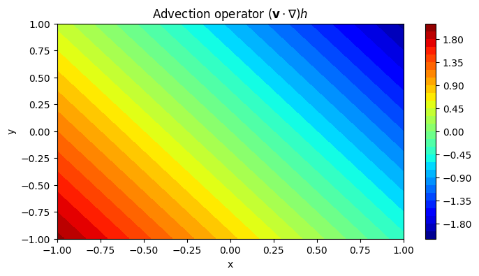

This plot tells us that as the height increases in the middle, the advection starts to drop towards zero. The advection variation is aligned with the velocity vectors shown in the plot prior. Beyond the height peak, the advection starts to decrease. To clarify, this plot is characterizing the rate of change of height based on the velocity held by a traveller.