Problem 1

Calculate the flow conditions downstream of a shock with the following upstream properties:

\[ \require{color} {\color[rgb]{0.041732,0.352132,0.699576}M_1} = {\color[rgb]{0.041732,0.352132,0.699576}1.5}, \; \; \; {\color[rgb]{0.315209,0.728565,0.037706}p_1} = {\color[rgb]{0.315209,0.728565,0.037706}100 \; kPa}, \; \; \; {\color[rgb]{0.164799,0.878862,0.723179}T_1} = {\color[rgb]{0.164799,0.878862,0.723179}300 K} \]

Assume the value of \(\gamma\) is \(1.4\).

cycle

(image above from An album of fluid motion by Milton Van Dyke)

Solution

We will approach this problem using two approaches. In the first approach we shall make use of the normal shock formulas. From Lecture, we know that

\[ \require{color} \large {\color[rgb]{0.041732,0.352132,0.699576}M_2}^2 = \frac{1 + \frac{\gamma - 1}{2}{\color[rgb]{0.041732,0.352132,0.699576}M_1}^2}{\gamma {\color[rgb]{0.041732,0.352132,0.699576}M_1}^2 - \frac{\gamma-1}{2}} \]

\[ \require{color} \large {\color[rgb]{0.041732,0.352132,0.699576}M_2}^2 = \frac{1 + \frac{1.4 - 1}{2}{\color[rgb]{0.041732,0.352132,0.699576}1.5}^2}{1.4 \times {\color[rgb]{0.041732,0.352132,0.699576}1.5}^2 - \frac{1.4-1}{2}} \]

This leads to

\[ \require{color} \large {\color[rgb]{0.041732,0.352132,0.699576}M_2} = 0.7011. \]

To work out the static pressure we have:

\[ \require{color} \large \frac{{\color[rgb]{0.315209,0.728565,0.037706}p_2}}{{\color[rgb]{0.315209,0.728565,0.037706}p_1}} = \frac{2 \gamma}{\gamma + 1} {\color[rgb]{0.041732,0.352132,0.699576}M_1}^2 - \frac{\gamma - 1}{\gamma + 1} \]

\[ \require{color} \large \Rightarrow \frac{{\color[rgb]{0.315209,0.728565,0.037706}p_2}}{{\color[rgb]{0.315209,0.728565,0.037706}p_1}} = \frac{2 \times 1.4}{1.4 + 1} {\color[rgb]{0.041732,0.352132,0.699576}1.5}^2 - \frac{1.4 - 1}{1.4 + 1} = 2.4583 \]

\[ \require{color} \large \Rightarrow {\color[rgb]{0.315209,0.728565,0.037706}p_2} = 2.4583 \times {\color[rgb]{0.315209,0.728565,0.037706}100 \; kPa} = {\color[rgb]{0.315209,0.728565,0.037706}245.83 \; kPa} \]

Finally, to work out the static temperature we use

\[ \require{color} \large \frac{{\color[rgb]{0.164799,0.878862,0.723179}T_2}}{{\color[rgb]{0.164799,0.878862,0.723179}T_1}} = \frac{\left( 1 + \frac{\gamma - 1}{2}{\color[rgb]{0.041732,0.352132,0.699576}M_1}^2\right) \left( \frac{2 \gamma}{\gamma - 1} {\color[rgb]{0.041732,0.352132,0.699576}M_1}^2 - 1 \right) }{\frac{\left(\gamma + 1 \right)^2}{2 \left(\gamma - 1 \right){\color[rgb]{0.041732,0.352132,0.699576}M_1}^2 }} \]

\[ \require{color} \large \Rightarrow \frac{{\color[rgb]{0.164799,0.878862,0.723179}T_2}}{{\color[rgb]{0.164799,0.878862,0.723179}T_1}} = \frac{\left( 1 + \frac{1.4 - 1}{2}{\color[rgb]{0.041732,0.352132,0.699576}1.5}^2\right) \left( \frac{2 \times 1.4}{1.4 - 1} {\color[rgb]{0.041732,0.352132,0.699576}1.5}^2 - 1 \right) }{\frac{\left(1.4 + 1 \right)^2}{2 \left(1.4 - 1 \right) \times {\color[rgb]{0.041732,0.352132,0.699576}1.5}^2 }} \]

\[ \require{color} \large \Rightarrow \frac{{\color[rgb]{0.164799,0.878862,0.723179}T_2}}{{\color[rgb]{0.164799,0.878862,0.723179}T_1}} = 1.3202 \]

\[ \require{color} \large \Rightarrow {\color[rgb]{0.164799,0.878862,0.723179}T_2} = 1.3202 \times {\color[rgb]{0.164799,0.878862,0.723179}300 \; K} = {\color[rgb]{0.164799,0.878862,0.723179}396.06\; K} \]

Alternatively, we can make use of the gas flow table; see below.

cycle

You will be provided these tables (or a relevant portion thereof) for solving such a problem. The one shown above is for supersonic flows, i.e., where the Mach number is greater than unity. A similar one exists for subsonic flows, however it has far fewer columns (see Problem 2) as it does not include any shock relations.

There are a few points to note regarding the columns of such a table. The first column is the Mach number, but just because it is supersonic doesn’t imply that there will be a shock. When there is no shock, the flow is still considered isentropic, and thus one can use the isentropic flow relations to work out static-to-stagnation ratios. This corresponds to the columns 2 to 4 (inclusive). The column with \(M_s\) and the four columns thereafter correspond to a scenario where there is a normal shock; the subscript \(s\) denotes shock. To clarify, \(M_s\) is the post-shock Mach number, \(P_{0s} / P_{0}\) is the ratio of the stagnation pressure post-shock vs the stagnation pressure pre-shock, and so on. The values we have computed above using the normal shock relations are highlighted and shown within rectangles for clarity.

Problem 2

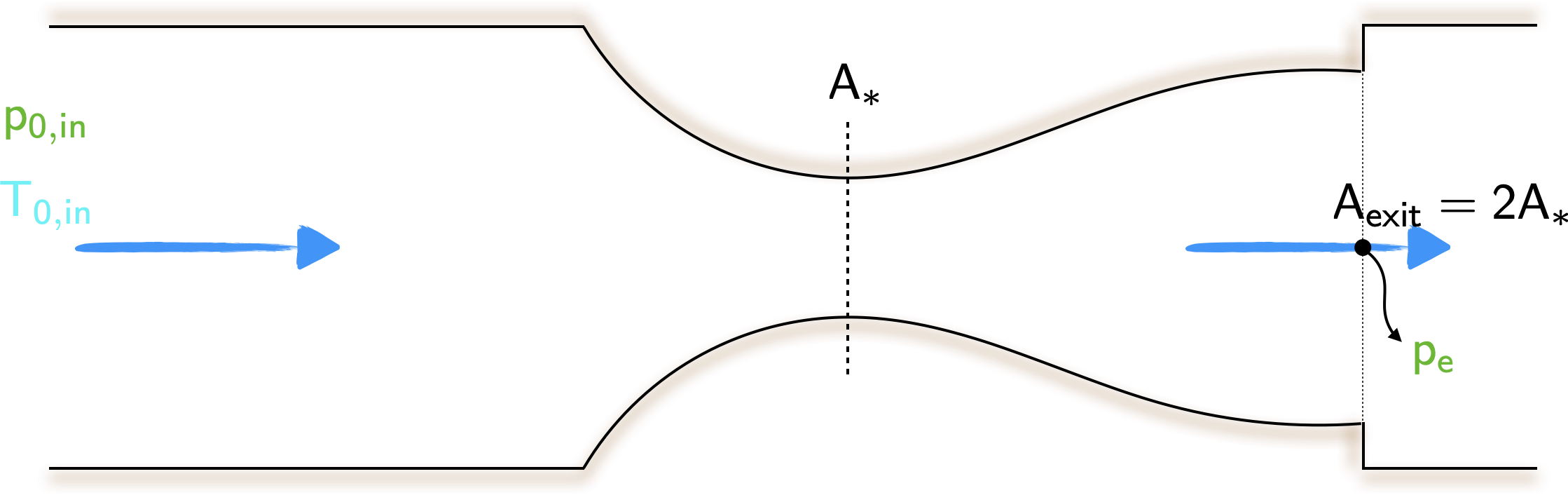
Consider the converging diverging duct shown below. The ratio of the exit static pressure to the inlet stagnation pressure is \(0.7\). Assuming the throat is choked and that there is a shock in the diverging section, calculate

  • the exit Mach number
  • the strength of the shock.

cycle

Solution

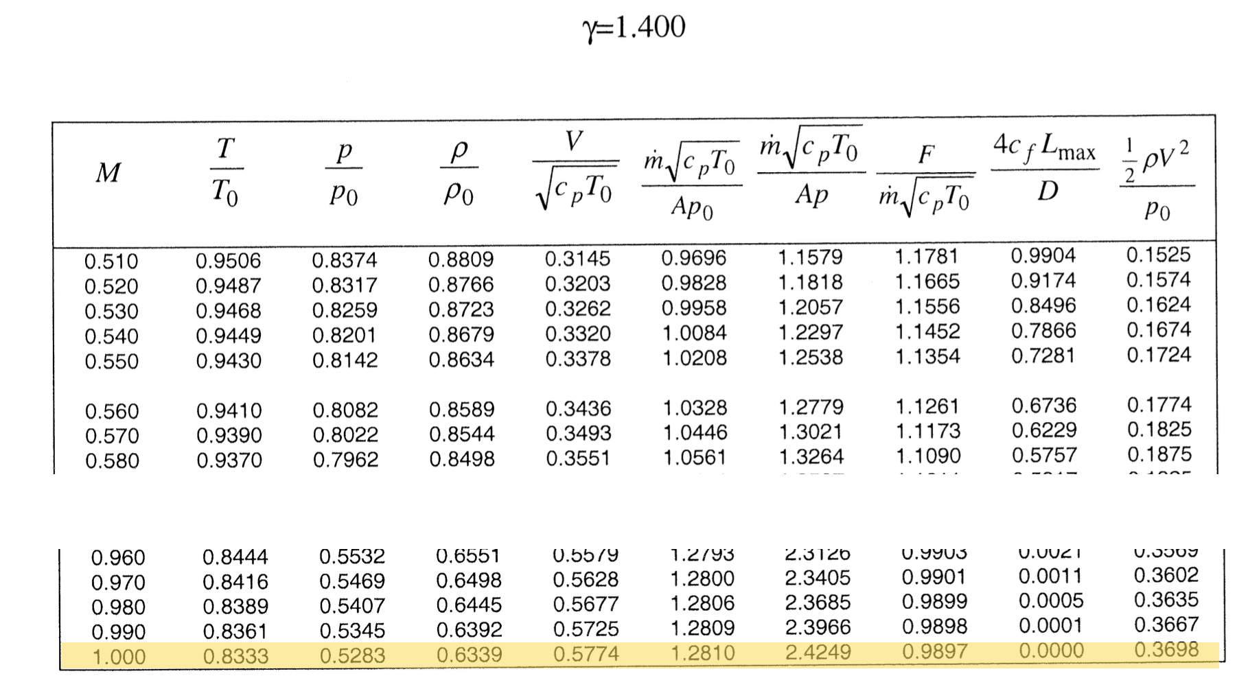
To begin, consider the last row of the subsonic tables. These are shown below.

cycle

Consider the column for the non-dimensional flow function

\[ \large \require{color} \frac{\dot{m} \sqrt{{\color[rgb]{0.986252,0.007236,0.027423}c}_{\color[rgb]{0.315209,0.728565,0.037706}p} {\color[rgb]{0.164799,0.878862,0.723179}T_0} }}{A {\color[rgb]{0.315209,0.728565,0.037706}p_0}} \]

One can imagine that as the area changes within a duct, the Mach number will also change. However, assuming there is no shock, the stagnation pressure will stay the same; the stagnation temperature will also stay the same (even if there is a shock). So will the massflow rate (conservation) and \(\require{color}{\color[rgb]{0.986252,0.007236,0.027423}c}_{\color[rgb]{0.315209,0.728565,0.037706}p}\). Thus, this column is useful for understanding the relationship between the area and the Mach number. From the highlighted row in the table, we can write

\[ \large \require{color} \frac{\dot{m} \sqrt{{\color[rgb]{0.986252,0.007236,0.027423}c}_{\color[rgb]{0.315209,0.728565,0.037706}p} {\color[rgb]{0.164799,0.878862,0.723179}T_0} }}{A_{\star} {\color[rgb]{0.315209,0.728565,0.037706}p_0}} = 1.281 \]

where \(A_{\star}\) denotes the area where the flow chokes. Given that the area at the exit is twice of the area at the throat, and given the pressure ratio we have

\[ \large \require{color} \frac{\dot{m} \sqrt{{\color[rgb]{0.986252,0.007236,0.027423}c}_{\color[rgb]{0.315209,0.728565,0.037706}p} {\color[rgb]{0.164799,0.878862,0.723179}T_0} }}{A_{exit} {\color[rgb]{0.315209,0.728565,0.037706}p_{exit}}} = \frac{\dot{m} \sqrt{{\color[rgb]{0.986252,0.007236,0.027423}c}_{\color[rgb]{0.315209,0.728565,0.037706}p} {\color[rgb]{0.164799,0.878862,0.723179}T_0} }}{A_{\star} {\color[rgb]{0.315209,0.728565,0.037706}p_0}} \times \frac{{\color[rgb]{0.315209,0.728565,0.037706}p_0}}{{\color[rgb]{0.315209,0.728565,0.037706}p_{exit}}} \times \frac{A_{\star}}{A_{exit}} \]

\[ \large \require{color} \Rightarrow \frac{\dot{m} \sqrt{{\color[rgb]{0.986252,0.007236,0.027423}c}_{\color[rgb]{0.315209,0.728565,0.037706}p} {\color[rgb]{0.164799,0.878862,0.723179}T_0} }}{A_{exit} {\color[rgb]{0.315209,0.728565,0.037706}p_{exit}}} = 1.281 \times \frac{1}{0.7} \times \frac{1}{2} = 0.915 \]

where note that the denominator has \(\require{color}{\color[rgb]{0.315209,0.728565,0.037706}p_{exit}}\) which is a static pressure.

cycle

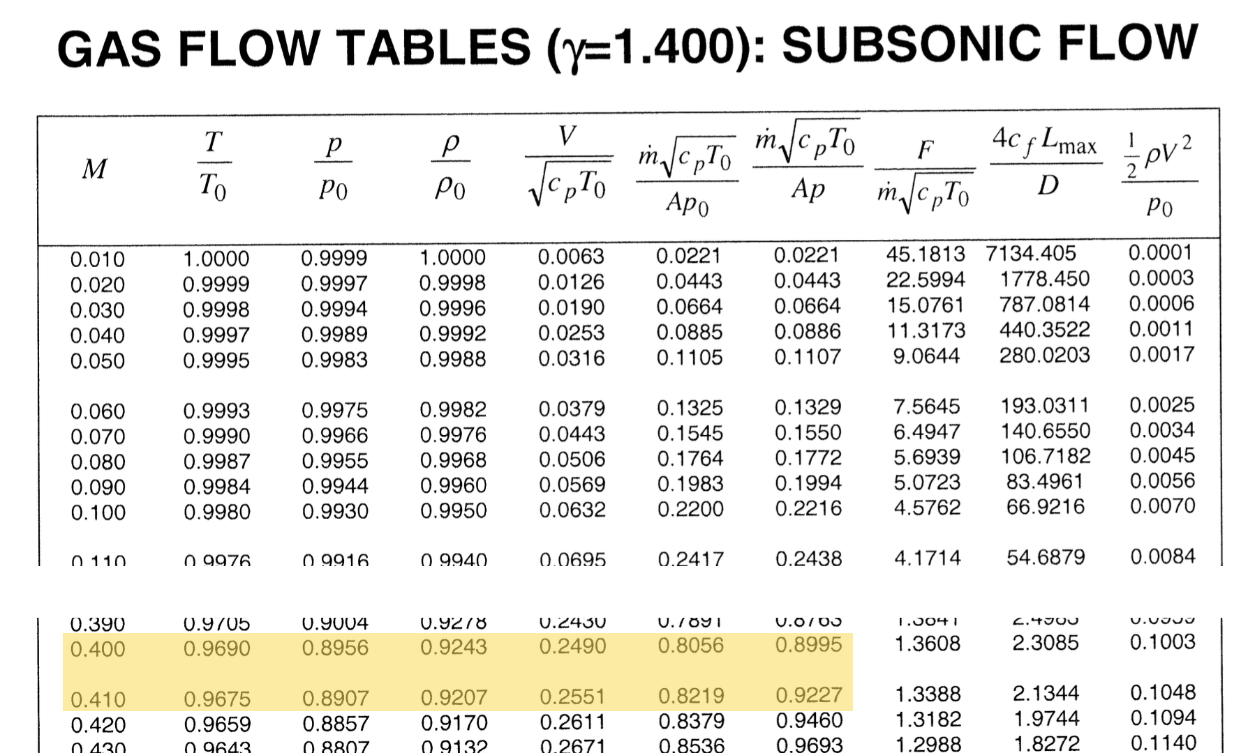
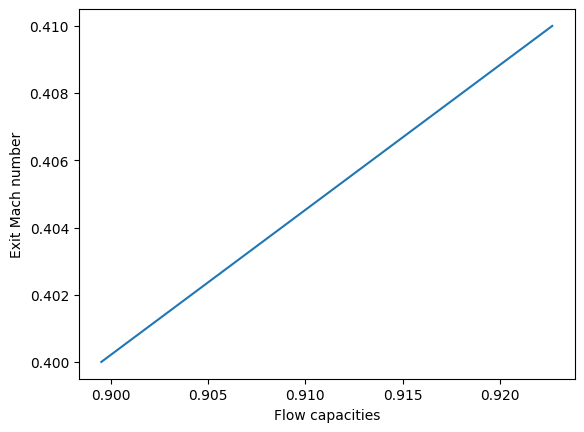
Using the tables again, we find that this value of \(0.915\) lies between \(0.8995\) and \(0.9227\), implying that the \(\require{color}{\color[rgb]{0.041732,0.352132,0.699576}M_{exit}}\) has values between \(\require{color}{\color[rgb]{0.041732,0.352132,0.699576}0.40}\) and \(\require{color}{\color[rgb]{0.041732,0.352132,0.699576}0.41}\). To work out exactly what this value is, we must interpolate; from the block of code below the corresponding exit Mach number is found to be \(\require{color}{\color[rgb]{0.041732,0.352132,0.699576}0.407}\).

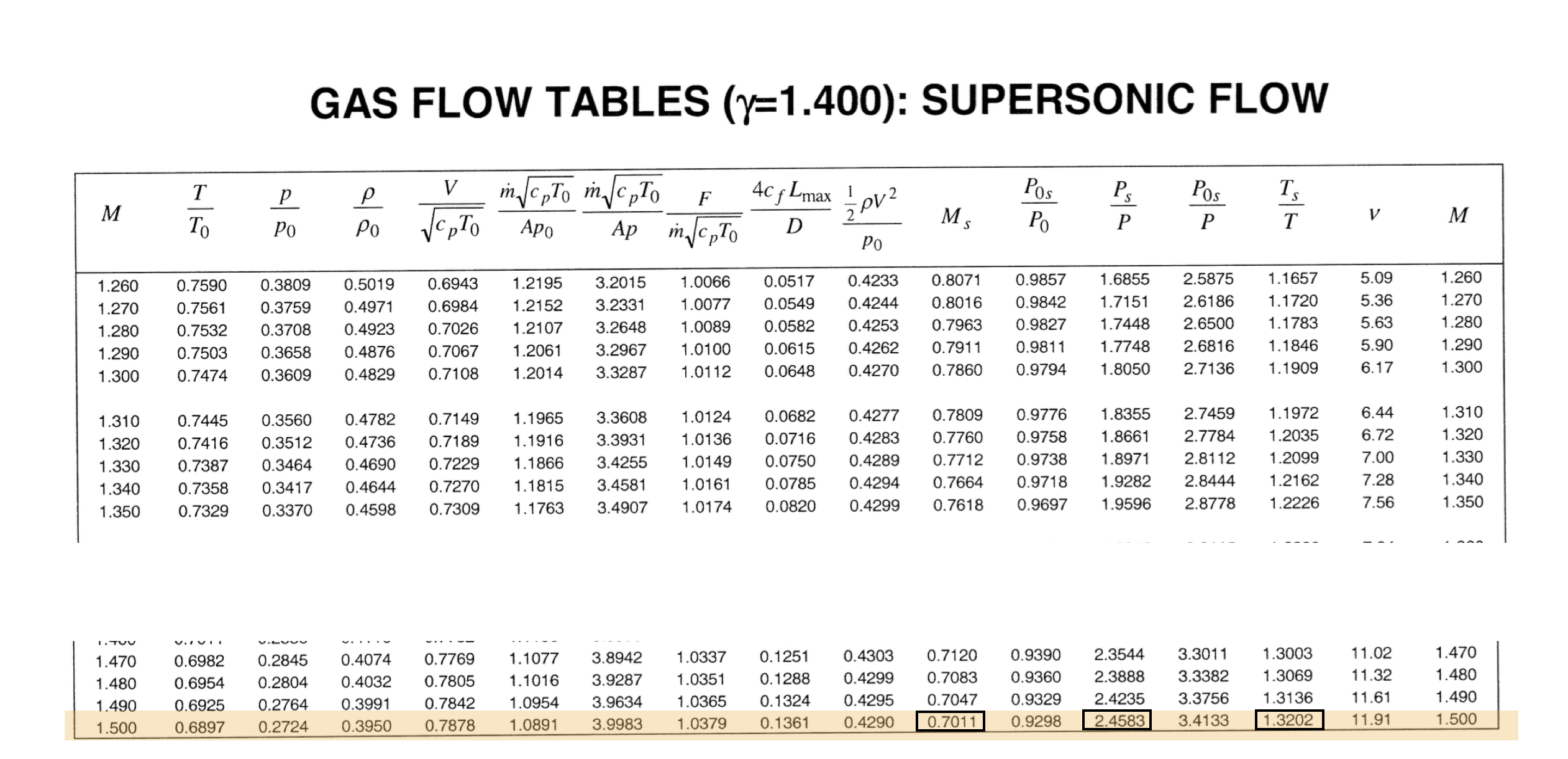
Next, to work out the strength of the shock, i.e., its Mach number, we recognize that across the shock there will be a drop in the stagnation pressure. The stagnation pressure downstream of the shock will be the same stagnation pressure at the exit.

\[ \large \require{color} \frac{{\color[rgb]{0.315209,0.728565,0.037706}p_{0,exit} }}{{\color[rgb]{0.315209,0.728565,0.037706}p_{0} }} = \frac{\dot{m} \sqrt{{\color[rgb]{0.986252,0.007236,0.027423}c}_{\color[rgb]{0.315209,0.728565,0.037706}p} {\color[rgb]{0.164799,0.878862,0.723179}T_0} }}{A_{\star} {\color[rgb]{0.315209,0.728565,0.037706}p_{0}}} \times \frac{A_{\star}}{A_{exit}} \times \frac{A_{exit} {\color[rgb]{0.315209,0.728565,0.037706}p_{0,exit}}}{\dot{m} \sqrt{{\color[rgb]{0.986252,0.007236,0.027423}c}_{\color[rgb]{0.315209,0.728565,0.037706}p} {\color[rgb]{0.164799,0.878862,0.723179}T_0} }} = 1.281 \times \frac{1}{2} \times \frac{1}{0.817} = 0.784 \]

Note that the stagnation pressure at the throat is the same as the stagnation pressure at the inlet. The value of \(0.817\) arises by interpolating between the two highlighted flow capacities (stagnation pressure in the denominator).

Finally, we can use this value of the stagnation pressure ratio to work out the Mach number of the shock, using the table below.

cycle

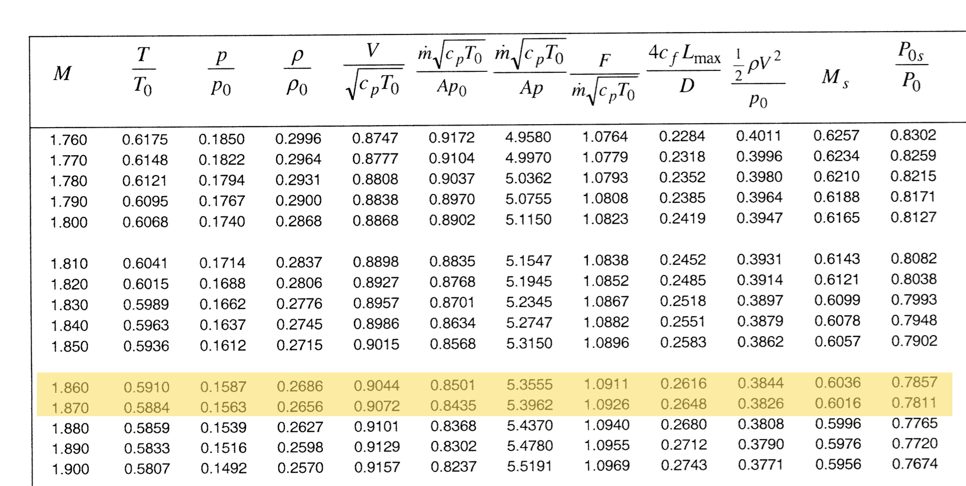
Studying the last column, we note that the Mach number of the shock has to lie between \(\require{color}{\color[rgb]{0.041732,0.352132,0.699576}1.86}\) and \(\require{color}{\color[rgb]{0.041732,0.352132,0.699576}1.87}\). With a spot of interpolation the value calculated is \(\require{color}{\color[rgb]{0.041732,0.352132,0.699576}M_{shock}} = {\color[rgb]{0.041732,0.352132,0.699576}1.867}\).

Code
# Block of code for linear interpolation
import numpy as np
import matplotlib.pyplot as plt

Mach_exit_A = 0.40
Mach_exit_B = 0.410
capacity_A = 0.8995
capacity_B = 0.9227
capacity_C = 0.915
slope = (Mach_exit_A - Mach_exit_B) / (capacity_A - capacity_B)
shift = Mach_exit_A - slope * capacity_A

capacities = np.linspace(capacity_A, capacity_B, 100)
Mach_exit = slope * capacities + shift


plt.plot(capacities, Mach_exit, '-')
plt.xlabel('Flow capacities')
plt.ylabel('Exit Mach number')
plt.show()

Mach_exit_C = slope * capacity_C + shift
print(Mach_exit_C)

0.4066810344827586